Getting into Digital Signal Processing: A Basic Introduction
Follow article
 Dave from DesignSpark
How do you feel about this article? Help us to provide better content for you.
Dave from DesignSpark
Thank you! Your feedback has been received.
Dave from DesignSpark
There was a problem submitting your feedback, please try again later.
Dave from DesignSpark
What do you think of this article?
Analogue Signal Processing
The real world is analogue! So why is every machine or instrument around us in the home or at work increasingly described as 'Digital'? To answer this question, we had better establish what we mean by the word: 'Analogue'.
All measurable things in life vary continuously in amplitude (size) with time: the outside temperature, the speed of a car or even daylight. We can convert a varying temperature to a varying electrical voltage using a sensor. We now have an electrical analogue of the original effect. As the temperature varies so does the voltage. Now we have this analogue signal, we can process it using other electronic components and display a temperature reading on a simple pointer instrument. The thing to remember is that natural parameters vary continuously, not in discrete steps; even devices that appear to operate in a discrete or digital manner can be deceptive.

Measuring the World
If we need to measure a length, we could use a ruler or tape measure. But what if we want a machine to take the measurement? Perhaps we would like the measurement displayed in different units according to a switch position, or even have the machine use the information itself and perform some appropriate action. We need an electrical or electronic system that converts whatever we are trying to measure to an electrical signal, maybe performing some signal processing before displaying or outputting the result.
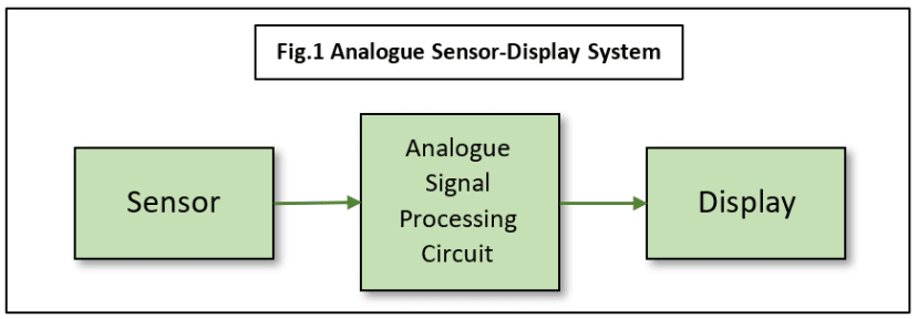
So, in summary, the component parts we need are (see Fig.1):
- Sensor(s), to convert the measured parameter to an electrical signal,
- A signal processing system, Analogue and/or Digital,
- Output Devices, to provide a Visual/Audio Interface to humans,
and perhaps
- Feedback for ‘Closed-loop’ or Automatic Control.
Simple Analogue Systems
A Single-Unit Measure-Display System requires no processing. Examples include the mercury thermometer, mercury barometer and the moving-coil ammeter. Notice that they are all ‘Analogue’ Systems, converting a parameter directly to a visible display.
The Two-Part Measure-Display System usually requires little or no processing and before cars became ‘digitalised’, examples of analogue measure-display could be found with the fuel gauge and water temperature instrumentation. In both cases, we have a separate sensor converting the parameter to an electrical signal, in these cases current, and a display instrument. The latter used a hot-wire method to convert the current value to a pointer position.
Measure-Process-Display Systems are more complex electronically than the examples above because some sort of signal conditioning circuits are included between the sensor and the display/output device. Traditionally these would be 'analogue' circuits composed of transistors, resistors, capacitors and more recently integrated circuits or 'chips'. Note that not all chips are digital. A typical piece of 'signal processing' might be to remove high-frequency electrical noise from a nearby electric motor. The circuit would probably be a Low-Pass Filter in this case.
What's wrong with Analogue Processing?
The systems discussed above a described as 'traditional' because they represent an era of measurement and electrical/electronic techniques that go back centuries. They had the advantage of being reliable and cheap to make (in large quantities). Analogue signal processing was kept to a minimum because electronic components were expensive, unreliable and required skilled design engineers to make it work. Let's look at this in more detail.
Component tolerances are a major headache for the analogue hardware designer. Very specific values of resistors or capacitors might be needed to realize a particular specification, but only certain preferred values are manufactured. This might mean resorting to variable components at greatly increased cost plus the need for setting up adjustments after production.
Component ageing is less of a problem nowadays thanks to new materials, but it can still be significant. For example, a resistor might have had a certain resistance value when it left the factory, but years later it may have changed enough to take the circuit outside its original specification or even to cause complete failure.
Electrical noise or Interference induced in the analogue circuit can sometimes be removed by additional circuitry if it can be distinguished from the wanted signal. More often than not, the electronics cannot tell the difference between noise and signal. Consider the old vinyl record player (now back in fashion for reasons that escape me): it’s impossible to remove the needle 'scratch', turntable bearing 'rumble', clicks, pops and hiss without removing chunks of the music as well. Your brain can sort it all out, but even the most sophisticated analogue processing system cannot. The best you can hope for is to reduce overall noise to an acceptable level.
Complex hardware design is needed for even simple processing tasks. Even if all you want to do is implement a low-pass filter, that is, remove all frequency components above a certain value from the signal, you will find it no easy task. Given a precise performance specification, there are a large number of possible techniques, each of which has an even larger number of possible circuit implementations. The tolerance problems come in to play, and if that wasn't enough, the layout and design of the printed circuit board (PCB) it's all built on may add 'stray' capacitance effects leading to instability in a high-frequency design. Design compromises are inevitable.
Difficulties in debugging, modifying, or updating an analogue hardware design cause the product to be expensive at the outset, with much wastage of effort later. Mistakes in the circuit design lead to the physical replacement of components and remaking of PCBs. Updates later on will often involve similar physical changes, so much so that usually it is not worth bothering and the whole system is designed again from scratch.
Digital to the rescue…
By now you could be forgiven for thinking that designing and making any new electronic system is fraught with such difficulty, that it's a miracle any 'high-tech' products are manufactured at all. Fortunately, salvation is at hand with the invention of the computer and Discrete-Time or Digital Signal Processing. In the 1920's work by a telegraph engineer called Harry Nyquist formed the basis of what we now call digital signal processing, although even he based his ideas on much earlier work by others. In order to realize the benefits of DSP, we must move from the Continuous-Time processing that we have been using up to now, to Discrete-Time processing.
What is meant by 'Discrete-Time'? Nyquist and others were able to show mathematically that you could work on samples of a signal taken at regular intervals and still get a satisfactory output. It seems bizarre, but it's true: you can sample a continuous waveform or signal, and then reconstruct the original continuous signal exactly from those samples. It gets better. The rule that governs this sampling, known as the Nyquist-Shannon Sampling Theorem, is very simple but without it there would be no digital signal processing. It’s not necessary to understand the complicated mathematical proof behind this very simple equation in order to use it:
fs > 2B where fs is the sampling rate and B is the bandwidth of the signal being sampled.
So, for example, if you have an audio signal with a maximum frequency limit of 15kHz, then you will need a sampling rate of more than 30000 samples/second. Naturally, there are one or two ‘catches’ which I’ll talk about later, but essentially if you sample the signal at this rate it is possible to recover the original analogue waveform exactly.
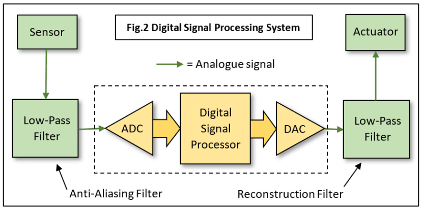
All we need is a device called an Analogue-to-Digital Converter (ADC) which takes a 'snapshot' of the signal voltage at regular intervals, converts this voltage level to a digital binary number and passes it to a digital computer which of course just loves binary numbers (Fig.2).
A simpler device known as a Digital-to-Analogue Converter (DAC) takes numbers from the computer and turns them back into voltage samples. The implications of all this are enormous….
Component tolerances and other hardware design problems almost disappear. This is because most of the analogue processing circuits are replaced by software algorithms running on the DSP chip. This makes debugging and updating potentially much simpler and cheaper because DSP systems are far easier to reprogram than analogue ones are to rebuild.
Ageing is now only a very long-term problem, and it too has a digital characteristic: the system either works to specification or it doesn't. Assuming that the software has been thoroughly debugged, the processing function will not change with time – unless it gets ‘hacked’. Security of embedded firmware is now a very real challenge with Internet-connected data acquisition systems becoming more common.
Noise problems are reduced. Audio CDs have none of the hiss and scratch of analogue tape and vinyl LPs because the sampled sounds are stored as digital data and are read back without any physical contact with the disc.
Practical Considerations
When it comes to designing a practical application based on DSP, it is of course, not that simple.
- The maths assumes a zero-width sampling pulse called a Dirac Delta Function. Unfortunately, it only exists in theory, and real finite-width pulses lead to predictable frequency distortion. But there are workarounds.
- The theoretical, perfect ‘brick-wall’ low-pass filter necessary to ensure the signal contains no frequency components above half the sampling rate is also impossible to make. We can work around this problem too. Note this analogue filter is needed before the ADC (Anti-Aliasing) and after the DAC (Reconstruction). See Fig.2.
- The ADC converts the signal into discrete levels, for example, an 8-bit ADC has a resolution of 256 levels. This introduces Quantization Noise which can be reduced by increasing the conversion resolution using a 12-, 16- or even 24-bit ADC instead. Many applications work just fine with 8-bits though.
Next Time
We’ll look at those practical workarounds mentioned above, including how to select the best sampling rate and design the corresponding anti-aliasing filter. Why is it called ‘anti-aliasing’ anyway?
If you're stuck for something to do, follow my posts on Twitter. I link to interesting articles on new electronics and related technologies, retweeting posts I spot about robots, space exploration and other issues.
Comments