Frequency Analysis for Embedded Microcontrollers, Part 4

Introduction

Part 1 and Part 2 provided an introduction to the theory behind the Discrete Fourier Transform and showed how input data must be processed to mitigate an effect called ‘Windowing’. Part 3 looked at running some actual code for the Microchip dsPIC33CH digital signal controller, and analysed the results. Now I’ll try and explain how the DFT evolved into the Fast Fourier Transform or FFT: the algorithm of choice for most engineers who need real-time spectral analysis of digitised waveform data.

The Fast Fourier Transform

The basic DFT algorithm is relatively simple to understand and code for a digital processor, but it was discovered as long ago as 1805 that it contained an awful lot of repeated identical calculations. Various people have come up with more efficient variants over the following 160 years, but it wasn’t until 1965 that two research scientists, James Tooley and John Tukey, put all this work together and came up with the definitive version of the FFT we know today. The FFT was developed to make more efficient use of the new and expensive (electronic) computing power that was becoming available.

DFT into FFT: The need for speed

The FFT is the DFT optimised for one thing only: speed. The improvement is normally characterised by the difference in the number of multiply operations that are required to transform N time-varying waveform samples into an N-point frequency spectrum.

For the DFT, N real multiply operations are needed to calculate each complex component of each output frequency point of the spectrum: X_R[k] and X_I[k]. That’s 2N operations for one frequency point. For the full spectrum (k=0 to N-1), the whole thing is repeated N-1 times yielding a final figure of 2N² for the DFT. That’s a lot, and it meant that when N became large, into the thousands, the raw DFT was impossibly slow when run on the early computer mainframes. On the other hand, its program code is easy to generate and follow. It consists of two nested DO loops (see Part 3); the inner one performs a dot-product and accumulate on N data samples to yield one frequency point, while the outer repeats the process N-1 times with the same data, but using a different set of sine-wave samples each time.

For the FFT, things are a bit more complicated. The basis of the algorithm is still the complex dot-product of a time-sample array and a sampled sine-wave array, but the sequence of operations has been completely rearranged to eliminate all the duplicated calculations. A core routine of the algorithm is the ‘Butterfly’ found in the innermost of three nested DO loops. It contains two complex multiplications needing four real multiply operations to be performed. The total number of operations for a complete set of N complex frequency outputs is 4Nlog₂N. Especially for large values of N, that represents a massive reduction in execution time compared to that of the same-size DFT.

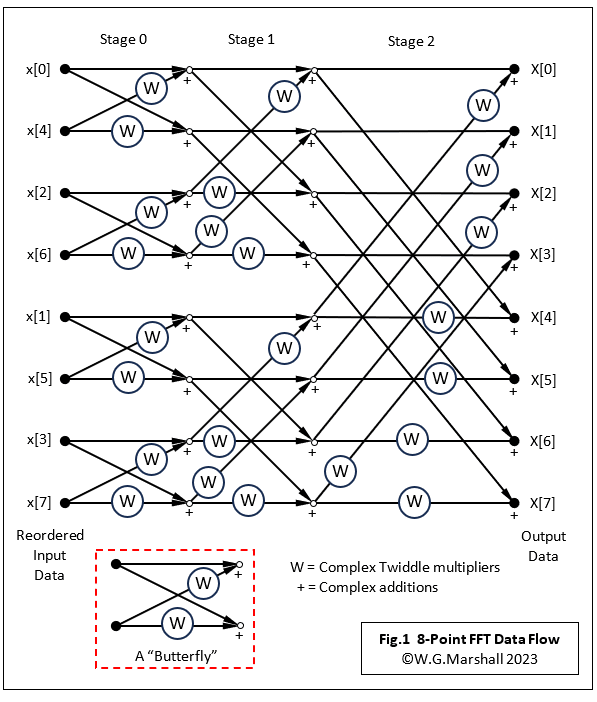
The thing about the FFT is that it’s not a completely new algorithm that rendered the DFT obsolete years ago. In fact, the fundamental mathematical principle behind it also drives the original DFT. I’m not going to attempt a detailed explanation of the FFT’s inner workings because the maths is just about impossible to visualise graphically. Besides, any book on DSP will have a chapter on the FFT; although I’ve not found one yet that doesn’t get bogged down in the literally complex mathematics. The basic principle involved is to start with an N-point DFT and split it into two N/2-point DFTs, one with the ‘even’ index numbers and the other with the ‘odd’. The outputs of the two smaller DFTs are combined with a few more complex multiplications and adds to yield a sampled spectrum output. This process actually results in a small reduction in the number of operations required. Further improvements can be made by further dividing the two N/2-point DFTs into four N/4-point DFTs and combining their four sets of outputs. Keep going with this until the logical conclusion is reached: N/2 x 2-point DFTs. The result is a massive reduction in the number of multiplications/adds required because so many of the DFT’s repeated calculations have been eliminated. Take a look at the data flow chart for an 8-point FFT algorithm (Fig.1). Each arrow is a complex number as are the W multipliers or ‘Twiddle’ factors. These W factors are the Sine and Cosine samples for a particular frequency index k and their multiplication with the complex data forms part of the ‘dot-product’ at the heart of the DFT.

Expansion to larger formats is easy. For example, the 256-point FFT I coded up for this article requires N/2 = 128 x 2-point butterflies for each stage and there are log₂N = 8 stages. Each stage contains N = 256 complex multiplications (or 4N real multiplications).

Speed improvement – at a price

All the duplicated calculations have been taken out of the basic DFT and we now have a really high-performance algorithm. No gains are ever free, so what is the cost?

• The input data sequence x[n] needs to be shuffled to separate the ‘even’ data points from the ‘odd’. It’s called ‘Decimation-in-Time’ or ‘Data Reordering’, and uses a Bit-Reversed Addressing routine to swap the data around (Fig.2). It represents a coding overhead not required by a DFT.

Fortunately, DSP chips such as the dsPIC33 have built-in bit-reversed addressing modes that allow a compact and fast DIT routine to be coded (Code 1).

• The FFT is nothing like as flexible as the basic DFT: it does one thing only, converting N samples of a time-varying waveform to an N-point frequency spectrum. It can, however, perform an inverse FFT with just a few minor changes. As mentioned in Part 3, a DFT can work with any size of data window. The FFT’s clever algorithm limits N to ‘binary’ lengths from 2 to 128, 256, 512 and so on.
• Both DFT and FFT produce ‘mirrored’ outputs. Only the first N/2 output samples are valid. The upper half of the results is just a reflected image of the lower half thanks to aliasing effects beyond the Nyquist limit. But, the DFT allows you to limit processing to the first N/2 frequencies thus halving the time taken to get a valid spectrum. With an FFT, you don’t have that option.
• Scaling. The 32-bit result of each multiplication is scaled by 15 bits (divided by 32768) to avoid arithmetic overflows. My dsPIC33 code for the DFT uses a similar, but more calculated operation after each Multiply-Accumulate (MAC). The FFT requires a further scaling function before each Stage is executed (Code 2). This checks the current REAL and IMAG data arrays for potential overflow and if detected divides the contents of both by two. The DFT scaling is much simpler because each real and imaginary frequency component of an output is created with just one MAC operation. The final output of the FFT only appears after the equivalent of 4Nlog₂N MACs have been completed!

A useful feature of the FFT is that it’s calculated ‘in-place’, meaning that no separate output data array is needed. Although modern DSP/MCU chips can have generous amounts of RAM available, the saving might prove critical with large FFTs.

The FFT Code

Finally, here is the code snippet for the FFT itself (Code 3). Something of a nightmare to follow (and create), you should be able to see how the three nested loops for Stage, Group and 2-point Butterfly correspond with the data flow components in Fig.1.

The complete test program can be obtained from the Downloads section below. Most of the peripheral items for scaling input data, windowing, and displaying results are the same as those used in the DFT program of Part 3.

Some test results

Here are some results from running my FFT code. The first is the analysis for an 8-cycle square-wave. It’s a bit different from the DFT output with the same input (Part 3), simply because I added a rudimentary square-root function to the display code. The amplitude of the harmonics is now in better proportion (Fig.3).  

Now here is an example of ‘spectral leakage’ caused by the non-integer number of square wave cycles in the capture window (Fig.4). Notice the twin peaks of the fundamental and the fifth harmonic straddling the actual frequency values of 10.667 and 53.333 respectively. BUT, the third harmonic only has one peak because it just happens to fall on an integer value – 32. The same thing happens with the ninth harmonic on 96.

This is the Hann-windowed version of the above. The window has significantly reduced the overall spectral leakage, but has added unwanted frequencies either side of the previously ‘clean’ third harmonic (Fig.5). These peaks have appeared because the central lobe width of the Hann frequency response is twice that of a rectangular window. See Part 2 for some more information on the effect of windowing.

Finally, we have the spectrum of a single, unipolar, 16-sample-wide rectangular pulse (Fig.6), with its Sinx/x shaped envelope. Note that the lobe widths are determined by the pulse width. So, as the pulse narrows, the lobes get wider. This particular effect has great repercussions when returning a sampled digital signal back into the analogue world via a DAC. See my article on this subject.

Speed comparison

After all this effort just how much faster than the DFT does it run? The average timings for the above test runs, including scaling, reordering, and magnitude calculation, are:

DFT (First 128 valid results only): 4470 μs

FFT (All 256 results): 710 μs

Next time in Part 5

Adding an analogue sampling input to capture blocks of real signal data. This is the first part of a project to make a useful real-time frequency analyser based on a MikroElektronika Clicker 2 board.

Not quite the end

A future article will feature the integration of this FFT code into my FORTHdsPIC-DC software running on the Microchip Curiosity board for the dsPIC33CH dual-core chip. It will run on the 100MIPS Slave core.

If you're stuck for something to do, follow my posts on Twitter. I link to interesting articles on new electronics and related technologies, retweeting posts I spot about robots, space exploration and other issues. To see my back catalogue of recent DesignSpark blog posts type “billsblog” into the Search box.