Frequency Analysis for Embedded Microcontrollers, Part 2

Introduction

Part 1 of this series provided an introduction to the theory behind the Discrete Fourier Transform and showed how complex maths can be translated into an algorithm easily coded for a DSP chip. But before getting down to detailed coding of the DFT, consideration must be given to mitigation of an effect called ‘Windowing’. This effect, which causes varying degrees of distortion in the output, is caused by the compromises made in converting the theoretical equations to practical ones.

Compromises

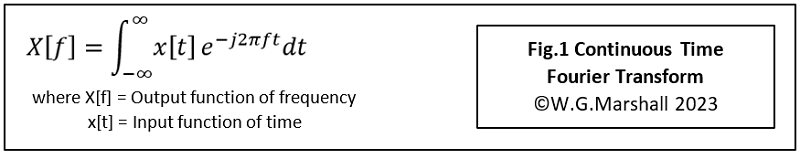
Appreciating, if not understanding, the first compromise requires a quick look at the original continuous-time Fourier Transform (Fig.1). Don’t panic, I’m not going to analyse the equation in detail; just point out one or two features.

This is a purely ‘theoretical’ equation illustrating a mathematical concept. It cannot be used to evaluate anything accurately in the ‘real’ world for fairly obvious reasons. For a start, there’s that integration sign with its limits of -∞ to +∞ (minus infinity to plus infinity). Surely infinity means ‘limitless’? How can you evaluate something that has no limit, and how can there be positive and negative infinity anyway? The term x[t] describes the input waveform between those ‘limits’. What we have here is an example of pure mathematical theory which is of no use to an engineer unless a way can be found to implement the equation with ‘real’ numbers. So, the first thing to do is convert the continuous time equation into a sampled or discrete format (Fig.2).

This is, of course, where we started in Part 1. Now we’ve gone ‘digital’, the rather frightening integration sign has been replaced by the much easier to handle summation sign: Σ. If at this point we keep the summation limits of -∞ to +∞, then we get what’s called the Discrete Time Fourier Transform (DTFT). Infinity is still an impractical concept, but at least it can show you what the ‘frequency envelope’ of the sampled waveform looks like with all possible frequencies present. For a practical analysis, we operate on a finite number of samples N instead, which provides a subset of the DTFT output. This version of the formula is called the Discrete Fourier Transform (DFT). In summary: for a given sampling frequency, the output envelopes of the DTFT and DFT will be the same: big main lobe with loads of sidelobes decreasing in size and stretching out to infinity. The difference is that the DTFT will encompass all possible frequencies present, whereas the DFT will only show a subset dependent on the window width N. So, that’s it, problem solved. Not quite, there is a reason why this paragraph is headed: Compromises.

Let’s look at the effect on the DFT output of a rectangular window applied to a single-frequency sine-wave (Fig.3).

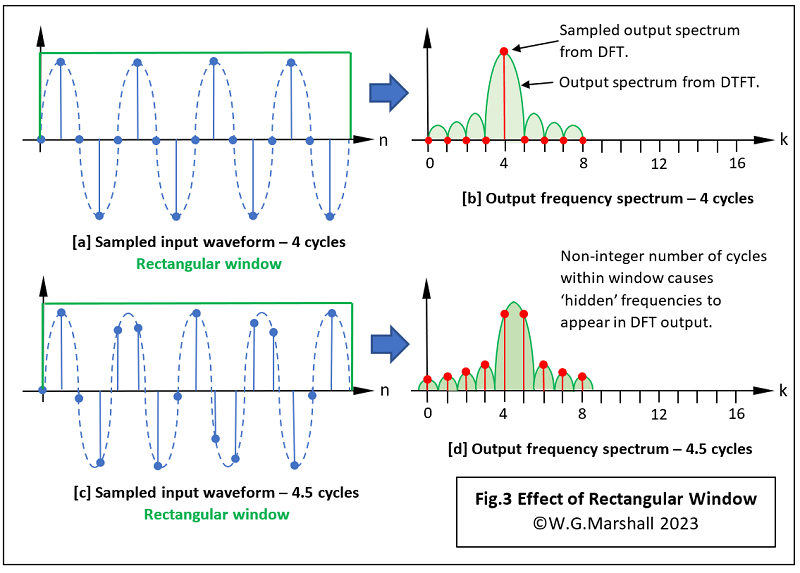
In Fig.3a, our 16-sample block or window, contains four complete sine-wave cycles: in other words, an integer number of cycles. Given that very simple input, the DFT comes out with the red sampled spectrum shown in Fig.3b. No surprise there; the only non-zero frequency component is at k = 4. But what about all those frequencies under the green (DTFT) envelope? They are ‘invisible’ artefacts caused by the sampling process, which don’t affect the DFT result because the latter’s sample points coincide with the sidelobes' zero-crossings. And that happens because the window contains an integer number of cycles. The window in Fig.3c is a non-integer example as it contains 4.5 cycles, leading to the distorted DFT result in Fig.3d. Once again, the green spectrum is not visible in its entirety, but this time its presence is made obvious by its effect on the DFT output in red. The green spectrum has moved to the right centring its main lobe over what should be k = 4.5. The DFT on the other hand, only works with integers and can’t produce a sample output in that position. Instead, you get two peaks of equal magnitude for k = 4 and k = 5. They are of equal size because 4.5 lies midway between 4 and 5. Further distortion or Spectral Leakage now appears because the DFT is sampling on the peaks of the green lobes rather than at the zero-crossings. Now imagine what the DFT output would look like if the input sample window contained many frequency components; some, if not all non-integer and randomly-phased relative to each other. What a mess. An alternative to the rectangular window shape may help.

Alternative Windows

A rectangular window produces the minimum mean-square-error estimate of the DFT compared with other shapes, but that’s not much use if you can’t see the wood for the trees, so to speak. How do you make a better window, one that lets the DFT reveal the frequency components of the input signal you want to see, while suppressing the others? All window types are a compromise, some working better than others with specific types of data. But all are designed to do two things:

• Eliminate the sharp discontinuity at each end of the rectangular window by ‘tapering’ the data samples to zero.
• Avoid introducing any discontinuities by employing a shape that changes smoothly along its entire width.

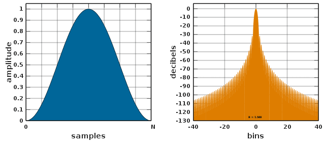
With one or two slightly oddball exceptions, most practical windows are based on the Cosine function. The Windows Function entry in Wikipedia contains a pretty comprehensive catalogue of shapes, but for most purposes the simple ‘Raised-Cosine’ or Hann window will suffice. As an aside, you sometimes find it mistakenly referred to in books as the ‘Hanning’ window. That leads to confusion with the very similar ‘Hamming’ design. You can see from the comparison in Fig.4 that use of the Hann window results in a considerable drop in the amplitude of the ‘side-lobes’ present in the output. The downside is that the main lobe is now twice the width. A ‘bin’ unit, as used in the frequency plots is defined as kf_S/N where f_S is the sampling frequency and N is the window length. In my examples, N = 16 so if we make f_S = 16Hz, then bin 0 covers 0-1Hz, bin 1 covers 1-2Hz and so on. I’ll talk about this a bit more when I describe the machine-coded DFT algorithms in a future article.

Applying the new window

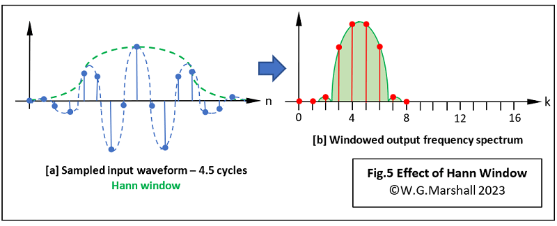
The new window has the same sample length as the input data block, or put another way, the same length as the original rectangular window. A dot product of the new window data set with the input data block is performed (without the summation). You can see the result in Fig.5a; note how the input data has been smoothly tapered down to zero amplitude at each end. Not a very good drawing, but the principle should be clear. The resulting frequency spectrum produced by the DFT is shown in Fig.5b. It’s a bit disappointing at first glance; the wider main lobe has exaggerated the immediately adjacent frequencies, but the much-reduced sidelobes have led to a sharp reduction in the more distant artefacts.

Next time in Part 3

In the next episode, I’ll produce some actual assembler code for the dsPIC, taking advantage of the chip’s DSP-specific instruction set and hardware. I’ll go through some practical applications, with some tips for window selection, and showing that there are situations where the DFT may work better than the ubiquitous FFT.

If you're stuck for something to do, follow my posts on Twitter. I link to interesting articles on new electronics and related technologies, retweeting posts I spot about robots, space exploration and other issues. To see my back catalogue of recent DesignSpark blog posts type “billsblog” into the Search box.