Frequency Analysis for Embedded Microcontrollers, Part 1

Introduction

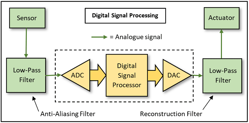
The algorithms for extracting the frequency components that make up a time-varying waveform have been around for decades. Until chip-friendly versions of AI algorithms (TinyML) took over, the most popular real-time code run on DSPs performed spectral analysis of complex waveforms, based on Fourier Analysis, specifically the Digital Fourier Transform or DFT. Although for various reasons I’ll talk about later, the most used form of the DFT nowadays is the Fast Fourier Transform or FFT. The original equations involved complex-exponentials and lots of integration, and remained largely a mathematical curiosity until they went ‘digital’ with the invention of the Nyquist–Shannon sampling theorem. This equation is very simple and underpins all digital signal processing. Essentially, it states that a continuous time-varying waveform can be fully reconstructed from discrete samples, providing that the highest frequency component present is less than or equal to, half the sampling rate. In other words: f_sample >= 2 x f_max. All DSP algorithms work with that basic assumption. The f_max is often referred to as the Nyquist Limit or Nyquist Frequency.

So why all the interest in real-time spectral analysis? Here are some practical examples:

• Making sure that a new design for an RF wireless transmitter does not emit frequencies outside the legal band limits.
• Detecting frequency components in the noise emitted by a machine that indicate wear with mechanical failure likely in the near future.
• Measuring the ‘frequency response’ of a hi-fi audio amplifier design to check that it’s ‘flat’ across the design bandwidth.
• Checking that a musical instrument only generates pleasant ‘odd’ harmonic frequencies of fundamental tones, rather than the unpleasant ‘even’ harmonics. Unless of course, it’s an electric guitar amplifier where second-harmonic distortion is essential when playing heavy rock music.

The Fourier transform is based on the assumption that any random, time-varying waveform can be ‘decomposed’ into a number of basic cyclic waveforms (so called ‘Sine’ waves), each possessing a unique frequency with a particular amplitude and phase relationship. It’s also reversable: given the right set of frequencies, the original waveform can be reconstructed.

Discrete Fourier Transform (DFT) reduced to multiplication and addition

The normal starting point for most articles on the DFT is the complicated mathematics of the original continuous-time (not sampled) theorem. What follows is not maths-free, but it’s worth the effort involved to understand the principles involved as they apply to some other powerful digital signal processing tools such as correlation, autocorrelation and FIR filtering. I’m allergic to integral signs so I’ll move swiftly on to the discrete-time version of the DFT:

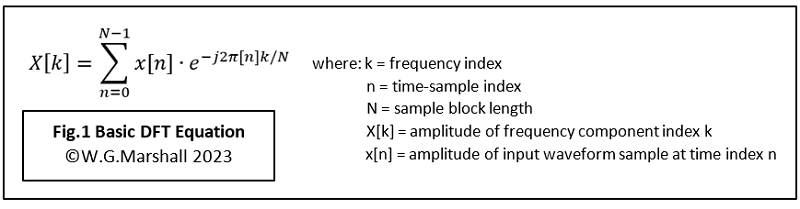
Yes, I know that’s fairly horrible too, but at least there’s no integral sign, this having been replaced by a sigma summation symbol, which just involves computer-friendly addition. The ‘e’ complex exponential is still there though, and that’s not friendly to computers or my brain. And then there’s that mysterious dot in the middle. Before I show you how to deal with the ‘e’, let’s take a look the core operation of the DFT involving the summation and the dot, known as a Dot Product.

Introducing the Dot Product

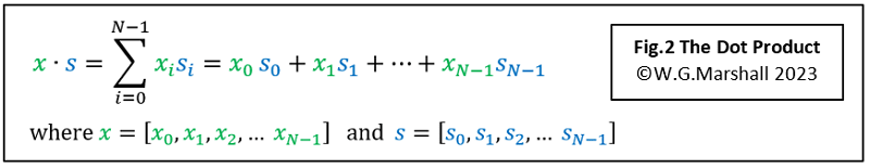
A vector is a sequence of numbers, such as a sampled waveform set. A dot product is what you get when the corresponding components of two vectors are multiplied together and the results added (or ‘Accumulated’) into a single number (Fig.2). Confusingly, the dot product definition shown includes the ‘sigma’ summation, but the DFT equations show it separately. This may be to make the latter easier to follow.

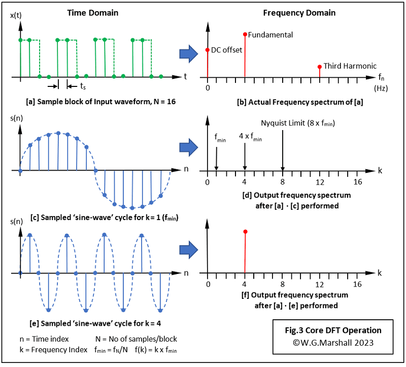
Now let’s apply the dot product to a sampled waveform x(t) of length N = 16 samples (Fig.3a), and a sampled reference ‘sinewave’ of the same length N (Fig.3c). I’ve deliberately chosen a very simple waveform for x(t) - four cycles of a 50-50 mark-space ratio pulse train, or ‘square-wave’ - because it contains very few spectral components (Fig.3b).

Calculating the lowest frequency component, f_min

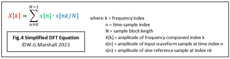
The minimum frequency component corresponds to k = 1. Plugging k = 1 into a simplified equation, Fig.4 (N is used to scale nk to keep it within the range 0 to N-1) and sweeping through all values of n from 0 to 255 will yield a near-zero magnitude for f_min.

Repeating this evaluation for k = 2 and k = 3 will generate the same result. Now try k = 4 (Fig.3e). This time we get a big peak (Fig.3f). That’s hardly a surprise: just compare Fig.3e with Fig.3a. The four reference cycles line up perfectly with the four square-wave cycles! Intuitively, a frequency of 4 x f_min must dominate the spectrum. Fig.3b indicates that the next frequency component in sequence is at k =12, or 12 x f_min, known as the 3^rd harmonic. The full spectrum contains all the ‘odd-number’ harmonics, theoretically right out to infinity.

The Nyquist Limit

Unfortunately, the Nyquist Limit described above prevents our short, N = 16, example from revealing anything above the ‘fundamental’ frequency at k = 4. That’s because the sampling rate f_s = N, so f_max = N/2 = 8 x f_min. This means that the largest value for k which gives a valid result is 8. Although for a square-wave, the amplitude of this frequency component is zero too. Hence, in general terms for a block of N time samples, the DFT will only produce N/2 + 1 frequency terms. The +1 refers to the zero-frequency or dc component.

The equation looks good so far, but you may have noticed an anomaly: there should be a component representing the dc-offset of the square-wave as it doesn’t swing equally positive and negative like the sine-wave reference. The dc or zero-frequency amplitude ought to appear when k = 0. But it doesn’t. It’s not difficult to figure out why:

When k = 0, nk = 0 for all values of n. And when nk = 0, Sin(nk/N) = 0

That’s one problem, and here’s another related issue: for the dot product to work, the sampled reference sinewave s(n) must align exactly with the corresponding sinewave ‘hidden’ within the sampled block x(t). But if it exists, it could lie anywhere within the block – it doesn’t even have to be aligned with the sampling points! The very simple square-wave we are using as an example input makes alignment easy, but complex waveforms require another approach. What’s needed is a method of establishing the magnitude of a spectral component without any prior knowledge of its position (relative phase) in the sample block.

Back to the drawing board

Not quite. I previously simplified the original DFT equation, replacing the complex exponential term with a single reference sampled sinewave (Fig.4). If you’ve got this far, you should have an understanding of the basic principle behind the DFT. Now we have to return to Fig.1 and use it to unlock the information needed to complete the transformation.

Euler’s Formula

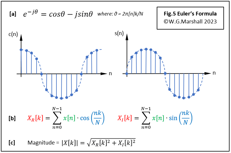
Evaluating that ‘e’ factor in Fig.1 will give us the magnitude of the selected frequency component, if present, whatever its position in the sample block. We can thank Leonhard Euler whose formula, (Fig.5a), translates the exponential into a more manageable form. It tells us that in addition to the dot product with a sinewave reference obtained already, another is required with the reference shifted by 90° - a cosine wave. So now we have two dot products for each frequency component (Fig.5b) labelled ‘Real’ (cosine) and ‘Imaginary’ (sine). At last, we have the core of the DFT ready for coding.

One last step

The two numbers define the relative magnitude of the selected sinewave component, and the phase – its position within the time sample block. Generally, it’s only the magnitude we are interested in, and that’s easily calculated by squaring and adding X_R and X_I (Fig.5c). The square-root is rarely implemented because it takes a lot of code to do it, and because the squared number is proportional to the signal power – a much more useful quantity.

Concluding points

It’s often said that the DFT is rendered obsolete by the Fast Fourier Transform (FFT) which has become a major feature of modern signal analysis equipment. The DFT is still very much alive: the FFT is just a DFT rearranged to reduce the number of operations by eliminating multiplications by 0 or ±1. Moving things around has the consequence of having to calculate the magnitudes of all k frequency components even if you’re only looking for one or two specific frequencies. In other words, the FFT is much faster if you want to generate a complete spectrum. On the other hand, an FFT will generate a full N+1 spectrum, but the high-frequency half will just be a mirror-image of the lower. Running a DFT with Real-only input data – the usual situation - you just calculate what you need.

If you’re new to DSP, and wish to understand the FFT algorithm, start with the DFT. After all, that’s how the people accredited with developing the modern FFT, Cooley and Tukey, started!

What’s next in Part 2

Before getting on to the subject of coding, there are some further ‘issues’ to consider. The ideal square-wave input I’ve used to illustrate the technique yields near-perfect results because it consists of an integral number of cycles (four), that fit precisely within the sample frame. The algorithm works because adjacent frames stretching either side of this one would be identical. The problem is that working on a grabbed frame from a complex, seemingly random waveform causes an effect called Windowing which leads to Spectral Leakage generating lots of extra, but erroneous frequencies in the output. Dealing with real-world data comes up in Part 2.

Although this type of algorithm can be, and is coded using a high-level language such as Python, for outright speed I prefer ‘bare-metal’ or machine code. The biggest headache with coding DSP algorithms is arithmetic overflow with all the multiply-accumulate operations needed. DSP chips like the Microchip dsPIC33 have all sorts of special instructions optimised for this type of code, and for ‘scaling’ those wayward numbers.

Bare-metal code development

Now that FORTHdsPIC-DC can load and execute code in the slave of a dual-core Microchip dsPIC33C series digital signal controller, and transfer data between cores, the time has come to look at serious applications, such as real-time frequency analysis. Some time ago I wrote a series of articles on the basics of digital signal processing which ended with some application examples such as digital filtering, and even AI (the perceptron). Having succeeded in running the latest version of FORTHdsPIC on the 90MIPS Master processor of a dsPIC33CH, I needed some computationally intensive code to run on the 100MIPS Slave. The development kit I’m using is the Microchip Curiosity board (187-6209) which features a couple of MikroElektronika ‘Click’ expansion sockets; handy because the previous version of FORTHdsPIC was developed on a ‘Clicker 2’ board, also with Click sockets!

If you're stuck for something to do, follow my posts on Twitter. I link to interesting articles on new electronics and related technologies, retweeting posts I spot about robots, space exploration and other issues. To see my back catalogue of recent DesignSpark blog posts type “billsblog” into the Search box above.