Frequency Analysis for Embedded Microcontrollers, Part 3

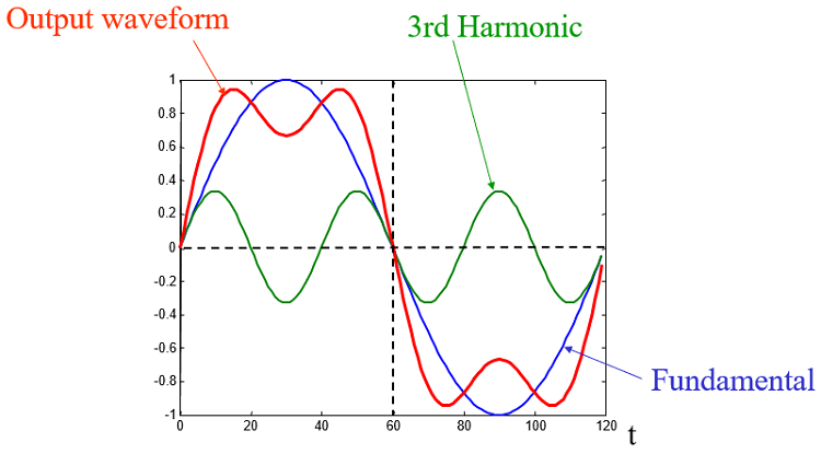
Waveform Synthesis: Adding sine-waves to make a square-wave.

Introduction

Part 1 and Part 2 provided an introduction to the theory behind the Discrete Fourier Transform and showed how input data must be processed to mitigate an effect called ‘Windowing’. Now let’s look at some actual code for the Microchip dsPIC33CH digital signal controller. The ‘CH’ variant is faster than the ‘E’ part and contains two processors: a Master running at 90MIPS and a Slave at 100MIPS. I used the Microchip Curiosity board (187-6209) for assembler-code development. The test program doesn’t work with real-time data; instead, the input arrays are filled with simple patterns that have known and easily recognised output spectra. Also, for testing purposes, the output data is not sent to a dedicated graphical display module, but to a virtual COM port emulator called Tera Term. The example spectra shown in this article are screenshots of the emulator window on the PC screen.

Designing the DFT

There is no ‘universal’ code for spectral analysis by Fourier Transform; an algorithm based on the formulas in Fig.1 needs to be constructed taking into account the range of frequencies in the output, and the frequency resolution required. Both of these parameters govern the choice of the Sampling Rate f_S, and the sample block size or Sampling Window Width N.

The Sampling Rate

Like all DSP systems working with sampled analogue data, the DFT only produces valid results from data that satisfies the Nyquist-Shannon sampling theorem: The sampling rate must be at least double the highest frequency component present in the waveform being sampled. So, in any design, the first job is to establish what that highest frequency is, and double it to get f_S. Chances are, your input waveform will have a much larger bandwidth than needed, so once f_S/2 has been determined, an analogue anti-aliasing filter with a sharp cut-off after this frequency should precede the ADC circuit.

Sampling Window Width

Having set the input sample period (1/f_S) to satisfy Nyquist, the next thing to do is decide on the output frequency resolution, or the frequency each output sample represents. This resolution is determined by the formula f_S/N. For the 256-point DFT example I use for the coding examples below, N = 256 and if f_S = 256 samples/sec, the frequency resolution is 1Hz making X(1) = 1Hz, X(2) = 2Hz, and so on up to X(255) = 255Hz. X(0) is always the zero-frequency or dc-offset component. But that leaves a problem: only X(0) to X(127) are valid because of the Nyquist sampling criterion. The rest are aliased, limiting the output frequency range to 127Hz. If a maximum frequency of 255Hz is specified and the resolution kept at 1Hz, then f_S and N must both be doubled to 512Hz and 512 respectively.

Program Sequence

Besides the DFT routine itself, other code blocks are needed to get a result. To start with, I’ll describe a DFT program which turns 256 samples of a time-varying waveform into a 128-sample frequency spectrum.

1. A block of N = 256 data samples must be loaded into the array REAL before any processing can begin.
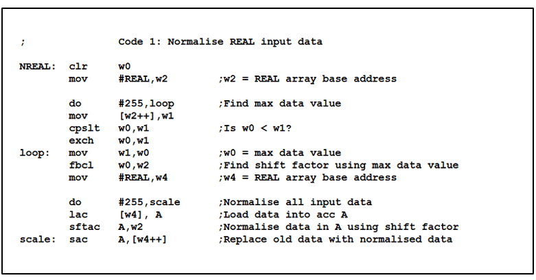
2. The input data is ‘normalised’ to take maximum advantage of the 16-bit number range of the dsPIC chip: -32768 to +32767.
3. The inherently ‘rectangular’ envelope to the block of samples can be altered to improve the result with some types of data. The envelope may be reshaped at this point by performing a dot-product (no summation) of the REAL data with a sampled version of the desired shape.
4. The REAL data is copied to the IMAGinary data array. Data obtained from an ADC is always considered ‘Real’. That’s why the input data sequence x(n) is the same for both X_R[k] and X_I[k] in Fig.1.
5. Use the DFT equations to find X_R[k] and X_I[k] for all values of k from 0 to (N/2) - 1. These results should also be normalised to retain accuracy.
6. Calculate the magnitude of each spectral component by combining the results of Step 5 using the magnitude equation in Fig.1. It’s usual not to bother with the square-root, leaving a result proportional to signal power instead.

The Code

A full listing of the assembler source code for the 256-point DFT can be obtained by clicking on the item in the Downloads section below. But here are some of the highlights.

(Step 2) This is a routine for normalising the input data to make maximum use of the signed 16-bit number format available. Normalising/scaling is carried out before, during, and after processing to ensure minimum loss of accuracy and, critically with integer-only working (i.e. not floating-point), to avoid overflows. The dsPIC instruction set has special functions to facilitate normalisation such as fbcl used in this routine which finds the first bit-change as it scans the word from the MS end. What this routine does first of all, is locate the largest number present in the data. The fbcl instruction then works out how many arithmetic shifts left (multiplications by 2) can be performed on it without causing an overflow. Once this is established, all the data items are shifted by this amount.

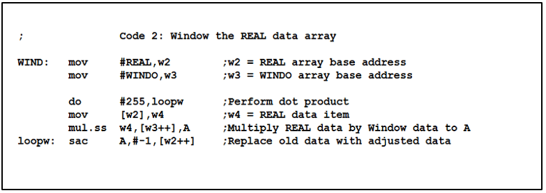
(Step 3) This short piece of code shapes or ‘Windows’ the block of time-sampled data in the REAL array with pre-calculated values from the array WINDO.

(Step 5) Finally, the core code that calculates the Real part of the output frequency spectrum, X_R[k] for k = 0 to 127. It consists of two nested loops. The inner loop calculates one X_R[k] result for each value of k supplied by the outer loop. At this point it should be noted that the DFT allows a single frequency component to be evaluated in isolation. In other words, if you want to establish that a particular frequency is present in a signal, then only the inner loop need be executed, supplied with the value of k corresponding to that component. This can’t be done with an FFT which requires the whole spectrum to be evaluated in one go. The code given here uses the outer loop to evaluate all the valid spectral components from k = 0 to 127. Having evaluated all the ‘Real’ X_R components, the whole process is repeated for the ‘Imaginary’ X_I output.

For a continuous, real-time display of a frequency spectrum, all the code from step 2 to step 6 must execute in less time than the sampling period 1/f_S. So, the faster those loops execute the wider the bandwidth of the analogue input signal that can be accommodated. DSP chips contain special hardware and an extended instruction set to help the designer meet the operating speed requirement of a particular application. A number of these features are used here.

• Zero-overhead DO loop instructions implemented in hardware. A major timesaver in most DSP applications. On the dsPIC33CH (and some EP) parts, DO loops can have up to four levels of ‘nesting’. The core DFT code here makes good use of two.
• Two 40-bit accumulator registers A and B. These help to reduce overflow problems when working with the looped Multiply-Accumulate operations frequently used in DSP applications.
• Single-cycle multiply, accumulate to A or B, and next operand fetch (MAC) instructions. When preceded by a REPEAT instruction, a MAC can realise an n-tap FIR filter in just n cycles.
• The instruction NORM, used in Code 3, drastically reduces the normalisation overhead.

Program output

The test program in the Downloads section below is a 256-point DFT working on a 256-sample-wide data capture filled with precisely 8 cycles of a bipolar square wave, otherwise known as a 50:50 mark-space ratio pulse train. I showed in Part 1 that this particular waveform contains very few frequency components and so is ideal for testing spectral analysis code. The first graph, Fig.2, shows the first 60 spectral lines of the DFT output with a rectangular window in place.

Unsurprisingly, the biggest peak is at k = 8, which is telling you that the fundamental frequency of a square wave is the same as its repetition rate. The next significant frequency is at k = 24 which is three times that of the fundamental, but much smaller in amplitude. It’s known as the Third Harmonic. Next is the Fifth Harmonic at k = 40 and so on, in theory, to infinity. In fact, just adding the fundamental frequency and the first three harmonics together will yield a perfectly useable square wave, if a bit ‘ripply’. Just one thing though: the ratio of their amplitudes to the fundamental must be correct. As it happens that’s easy. The third harmonic must be one-third the size of the fundamental, the fifth harmonic one-fifth, and so on. Oh dear, the numbers on the Fig.2 graph don’t add up. Actually, they’re pretty close, when you remember that each represents the amplitude squared. Comparing the square-roots of these numbers produces a much more satisfactory result. The second graph Fig.3, shows what happens when a Hann (Raised-Cosine) window is applied to the same 8 cycles of a square wave.

In this instance, it would appear that the application of the Hann window has added spurious frequencies, and very definitely not improved the result! Where these unwanted frequencies come from and why they appear was discussed in Part 2. Suffice to say that the ‘sidebands’ on either side of the correct frequencies are caused by the Hann window. At least the ‘correct’ frequencies are still obvious, but that is only because the input waveform is very simple with an integer number of cycles in the sample window – a feature not often encountered with real-world waveforms. However, when frequency components are few and well-spaced, the rectangular window will provide the best resolution. Now the next two graphs, Figs.4 and 5, feature the square-wave input again, but the input is not composed of an integer number of cycles; this time it’s 7.5 in a reduced window of 240 samples.

Looks pretty close to Fig.3 doesn’t it? Except for the single frequency peaks at k = 8, 24, 40 etc. being replaced by pairs at 7/8, 22/23 and 37/38. The algorithm cannot display the frequency at 7.5, 22.5 and 37.5 because only integer values of k are allowed, showing the nearest integer values on each side instead. Note also the growth in the components around the base of each harmonic pair. Both these effects are caused by spectral leakage as discussed in Part 2. Let’s see what happens when a Hann window is applied to this data in Fig.5.

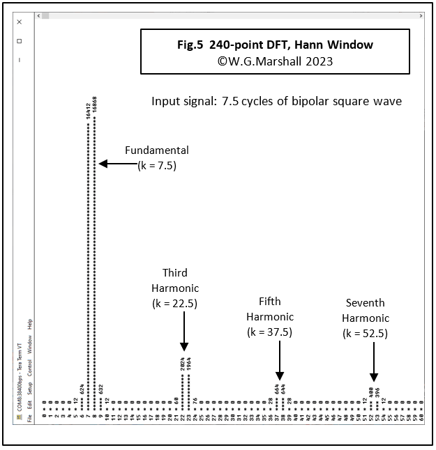
Now that looks much better than Fig.4. The tapering-off at the edges of the raised-cosine window has mitigated most of the effects of spectral leakage; the spurious frequencies at the base of the fundamental have been reduced. But nothing can change the fact that the DFT cannot ‘see’ frequency components that have a non-integer number of cycles across the width of the sample window, so the pairs of frequencies remain as markers thanks to the ‘centre lobe’ of a Hann Window frequency response being twice the width of a Rectangular.

Real-World Data

On the face of it, the DFT (and its faster sibling, the FFT) offer a neat way of extracting the frequency components that make up any time-varying waveform. In practice, the results can be hugely misleading. The simple square-wave example I’ve been using contains few significant frequency components, but imagine a complex waveform with many frequencies and phase relationships; very few with integer numbers of cycles within the chosen sampling window. I’m afraid the combined effects of all the spectral leakage will lead to a confused output that bears no relation to reality. What can be done? In an embedded application, it’s unlikely that you will want a full-spectrum readout. Most likely, the ability to detect/measure the presence/magnitude of one or two specific frequencies is all that is required. Assuming these frequencies are known from experiments done in the lab, then f_S and N can be tailored to give the best results. Windowing can be applied to reduce spurious peaks, but this will involve extensive experimentation to find the best algorithm. Many windows have been formulated in the past to suit particular applications; a number are described here. It may also be worth spending some time designing a powerful band-pass analogue anti-aliasing filter to block out all other frequency components – even those still within the Nyquist limit.

Only a DFT can be tailored to work with individual frequencies, unlike an FFT which is faster because it eliminates redundant operations but has to produce the full spectrum output. A DFT working on just a few frequencies is much, much faster. Another advantage of the DFT is that it will work on data blocks of any length. The FFT is limited to ‘binary’ lengths such as 128, 256, 512, 1024, and so on.

Speeding it up

An obvious thing to do is keep the number of block samples as low as possible while meeting the specification for accuracy and resolution. Another is to try and reduce the code within the DFT inner loop. A deeper understanding of how the code works can often yield dividends. For example, in the Code 3 snippet, you will notice that the divide k*n by N step is performed by a conventional unsigned divide instruction: DIV.U  w0,w2 which needs to be executed 6 times to get a result. That’s why it’s preceded by REPEAT  #5. A divide on an MCU is always slower than a multiply, in this case taking six machine cycles to the multiply’s one. These six cycles can be reduced to one with a ‘trick’ involving the block length first being limited to a value of 256. Now replace the repeat and div instructions with AND  #0x00FF,w0. Also replace the following SL  w1,w11 with SL  w0,w11. To understand how it works you need to know that the remainder from the DIV instruction is the important bit, not the quotient. I love tinkering with ‘bare-metal’ code like this – it can be very rewarding, on this occasion yielding a useful speed-up of a critical routine.

Next time in Part 4

I'll cover the Fast Fourier Transform (FFT) algorithm in some detail and include a dsPIC33 machine-coded version to allow a speed comparison with my DFT code.

If you're stuck for something to do, follow my posts on Twitter. I link to interesting articles on new electronics and related technologies, retweeting posts I spot about robots, space exploration and other issues. To see my back catalogue of recent DesignSpark blog posts type “billsblog” into the Search box.