Programming a DSP-based Digital Filter: Impulse Response

Here is a ‘scope picture showing the filter program in action: input to a dsPIC analogue (ADC) port on the bottom (blue) trace, output from the DAC on the top (yellow) trace. Sampling rate f_s = 524.288 kHz, cut-off f_c = 32.768 kHz, input = 5 kHz square wave. Number of Tap-gains = 59. The frequency spectrum of a square wave only contains a fundamental plus 'odd' harmonics. Notice that the fundamental (5 kHz) and 3^rd harmonic (15 kHz) are present in the output, but everything else is filtered out. The 5^th harmonic (25 kHz) and above have been lost in the roll-off before and after the cut-off frequency of 32.768 kHz. The program runs on a MikroElektronika Clicker 2 dsPIC33E board (144-8343) with a Click DAC board (820-9836) providing the analogue output.

Being Impulsive

At the end of Part 6 of my series on real-time signal analysis for embedded systems, I showed how the frequency spectrum of a single pulse had a sinc(x) or sin(x)/x envelope to it. In Fig.3 of that article, it’s possible to see how the ‘lobes’ get wider as the pulse narrows in width until the main lobe is so wide it appears as a flat line until well past the Nyquist frequency (f_s/2). At that point, the pulse is as narrow as it can get – just bigger than the sample period (1/f_s). So what, you say? Well, a particular form of this narrow rectangular pulse is the Dirac-Delta function which has a constant area: the pulse becomes taller as it narrows in width.

In the limit, as the mathematicians would say, the ‘ideal’ sampling pulse is created with zero width and infinite magnitude. This impulse thus contains all possible frequencies from -∞ to +∞ (Fig.1), which when applied to the input of, say, an analogue low-pass filter with a cut-off frequency f_c will produce an impulse response waveform at the output, as in Fig.2. Mathematically, this is the unnormalised sinc function with the definition:

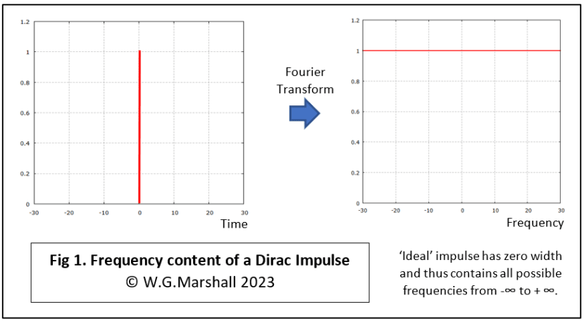
sinc(x) = sin(x)/x is true for all values of x except x = 0. At the latter point, the function features a divide-by-zero situation which is of course invalid. The x-axis zero crossings of the sinc function are at all non-zero integer multiples of π.

Or more usually with DSP applications, the so-called normalised version is used:

sinc(x) = sin(πx)/πx is also true for all values of x except x = 0. The zero crossings of this sinc function occur at all non-zero integers.

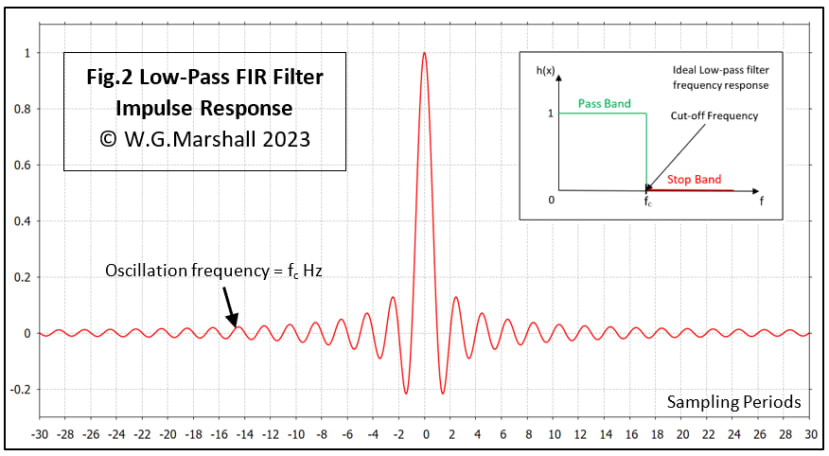
A mechanical analogy involves a hammer striking a bell: the hammer blow (or impulse) produces a loud sound causing the bell to ‘ring’ or resonate at its natural (resonant) frequency. After the impulse has gone, the bell continues to resonate, the sound intensity dying away gradually with time. That’s what is happening when the electrical impulse ‘strikes’ the filter input and the output continues to oscillate at the cut-off frequency f_c – theoretically forever in the ‘ideal’ case described.

The ideal low-pass filter will pass all frequencies up to f_c, but nothing higher, hence its being described as a ‘brick-wall’ filter. Some things to notice in Fig.2:

• That the waveform is symmetrical about zero on the time axis, extending into the ‘future’ as well as back into the ‘past’. This seems like it might be a serious issue with any practical realisation. Fortunately, it isn’t, because it just appears as a delay corresponding to the filter length between the input and output data samples in a digital FIR implementation.
• That the waveform is truncated on each side and doesn’t extend to infinity. Obviously, that’s why the digital version is called finite impulse filter. Now that does have a consequence that’s not easily resolved – the filter’s frequency response will not be brick-wall. Instead, the cut-off will be more of a roll-off and there may be ‘ripples’ in both the pass and stop bands.
• That the impulse response before and after the main lobe at t = 0 consists of a decaying oscillation at the cut-off frequency f_c.
• It’s not obvious, but the value of the function at x = 0 is missing in Fig.2 because of that divide-by-zero problem mentioned above. It doesn’t matter here, but a sensible value for it must be found when the function is ‘sampled’ to derive digital filter ‘tap-gains’ later.

The thing is though, you don’t use the impulse response to design an analogue filter, active or passive. So, what’s this all about then? It’s a useful introduction to the digital Finite Impulse Response (FIR) filter, which as its name suggests, is built around the impulse response.

Going Digital

Before moving on to describe the construction of a low-pass digital filter, I use the word construction because the algorithm can be realised both as software code running on a DSP chip, or hardware using latches, multipliers and adders. You can see how either method is possible by looking at the graphical representation of the algorithm in Fig.3. Here we have a basic 3-tap, or 2-pole FIR filter, which takes digitised samples x(n) from an ADC at a sampling rate of f_s and delivers output samples y(n) to, say, a DAC for conversion back to an analogue signal. The filter characteristic, i.e. cut-off frequency, high- or low-pass, is determined by the multiplier or Tap-Gain values a₀, a₁ and a₂. The use of the parameter ‘pole’, the latter defined as (No. of Taps) – 1, allows performance comparison with analogue filters. Crudely, for both analogue and digital, the more poles you have, the steeper the roll-off at the design cut-off frequency f_c. Though every additional pole in the analogue design means more non-trivial hardware complexity.

An FIR filter implemented in hardware requires a lot of extra hardware too, so clearly a reprogrammable software approach seems to be the way to go. Until the first DSP chip appeared in 1980, real-time operation at useful frequencies was way beyond the capability of microprocessors or microcontrollers at the time. As regular readers will know, I’m a fan of the Microchip dsPIC33 Digital Signal Controller, as the manufacturers insist upon calling it, and that is what I’ll be using to demonstrate the FIR filter in the next instalment. In the meantime, here is the code routine that implements a 61-tap version of the algorithm shown in Fig.3:

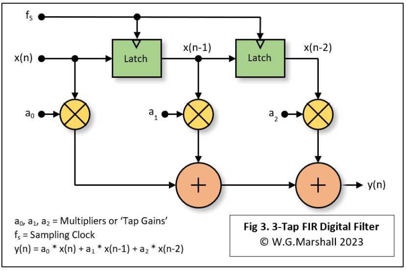
This routine runs once for every incoming data sample from the ADC, and outputs each time a processed data sample to a DAC. Not only must it fit into one interval of the sampling clock, 1/f_s, but so must the ADC sample capture and the DAC output routines! In practice, I’ve found that the whole code loop can execute fast enough to enable the 70 MIPS dsPIC’s ADC to be run flat-out at just over 1MHz.

If the functions shown in Fig.3 were to be implemented in hardware directly, the latches and adders could be made from TTL or CMOS logic parts, but the multipliers would pose more of a problem.

The Filter’s Impulse Response

Whether you go for a hardware-only or a DSP/software approach, one task is shared by both: establishing how many taps are required to achieve the desired performance and their tap-gain values. It should come as no surprise that this information can be derived from an examination of the sampled impulse response of the filter, created from the key parameters: data (ADC) Sampling Rate f_s, and the desired Cut-off Frequency f_c. Now look at Fig.4, but don’t panic if it looks a bit daunting.

Firstly, in this digital world, it makes life easier if we ‘normalise’ the cut-off frequency to the sampling rate, and call this number the Transition Frequency f_t:

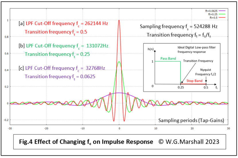
f_t = f_c/f_s     A dimensionless ratio.

This allows us to specify the cut-off point as a proportion of the sampling rate. So, for the three examples in the diagram:

[a] f_t = 0.5 and the cut-off frequency f_c is at its maximum value, i.e. the Nyquist frequency of 262144 Hz, or 0.5 x sampling rate f_s of 524288 Hz.

[b] f_t = 0.25 and the cut-off frequency f_c = 131072 Hz, or 0.25 x sampling rate f_s.

[c] f_t = 0.0625 and the cut-off frequency f_c = 32768 Hz, or 0.0625 x sampling rate f_s.

Using this normalised frequency f_t, the impulse response equation for the filter becomes:

h(x) = sin(2πf_tx)/πx for all x, except x = 0 when h(x) = 2f_t

How many Taps?

Now we come to the tricky bit of designing a digital filter. Implementing the basic algorithm is a straightforward task (see code above). The problem is deciding how many tap gains to use: too many in the pursuit of a ‘brick-wall’ cut-off, means it may not be possible to process each sample fully within the sample period 1/f_s. Too few, and slow roll-off, with ‘ripples’ both in the pass- and stop bands may lead to poor performance. I’ll talk about these trade-offs next time, but for now let’s consider how they are derived from the filter’s impulse response.

In principle, just sample the impulse response at the sampling frequency for the desired number of taps, and that’s it. Well, first of all, you need to determine how many taps are required to get the best possible roll-off at the desired cut-off frequency f_c. In Fig 4, 61 taps are used; that’s 30 negative, 30 positive, and one at x = 0 with the value 2f_t. Looks about right for these three cut-off frequencies. But there is still a sharp ‘step’ at -30 and +30. You could increase the number of taps, but that might exceed the processing limit of the DSP. An alternative is to apply a technique used to taper the ends of the sample blocks being processed by an FFT algorithm – Windowing. A Hamming raised-cosine window, for example, is applied to the array of tap-gains in the same way to smooth it down to zero at a(-30) at one end and a(30) at the other. Inevitably, a certain amount of trial and error is used to get the desired performance; I use a special program to set up an array of frequency samples that describe the desired filter frequency response. This is run through an Inverse FFT to reveal the sampled impulse response (tap gains) needed to provide it. At this point, you can just truncate the sequence or apply the window to smoothly reduce the outer taps to zero. The result is run back through the FFT to see what the resulting frequency response looks like. If unacceptable, try again with a different number of taps.

Next time

I’ll describe the tap-gain generator program in some detail and go over the full filter program highlighting its dsPIC features: as well as DSP-specific instructions like multiply-accumulate (mac) other useful facilities include modulo addressing for the creation of circular buffers.

If you're stuck for something to do, follow my posts on Twitter. I link to interesting articles on new electronics and related technologies, retweeting posts I spot about robots, space exploration and other issues. To see my back catalogue of recent DesignSpark blog posts type “billsblog” into the Search box above.