Give your Robot the Mobility Control of a real Mars Rover: Part 1
Follow article
 Dave from DesignSpark
How do you feel about this article? Help us to provide better content for you.
Dave from DesignSpark
Thank you! Your feedback has been received.
Dave from DesignSpark
There was a problem submitting your feedback, please try again later.
Dave from DesignSpark
What do you think of this article?
Robots, particularly the wheeled variety, can be divided into two classes: those that navigate around solely by sensing and avoiding obstacles, and those that move along a planned path using an internal electronic map. Most ‘hobby’ mobile robots tend to move about just using obstacle sensing. That’s a somewhat simplistic view based on the idea that rushing around avoiding things is a lot more fun (and easier) to program than accurate movement on a predetermined course!
Mobility Control
A ‘Professional’ robot, for example the Mars rover Curiosity, needs to navigate with precision, while at the same time avoiding large rocks and small craters.

To get an idea just how complex robot mobility hardware/software can get, have a look at this paper on the mobility system for Curiosity’s predecessors, the Mars Exploration Rovers Opportunity and Spirit. The block diagram, Figure 2 on page 3 of the paper describes the basic navigation system: this article and the next will describe what goes on in that block marked MOT, and how (and why) it’s functionality based on the PID algorithm can be added to a less exotic robot on planet Earth.
PID Control
The basic principle of PID control is very easy to understand and can be applied to any system involving an electro-mechanical actuator (e.g. a motor) which needs to be driven at a set speed or moved to an exact position. The extra hardware required consists of a sensor which provides data on the actual speed or position of the actuator, and a processor unit to run the control algorithm. The processor compares the desired mechanical output (set-point) with the sensed actual value and generates a modified control signal to cancel any difference (error). This algorithm is not limited to moving systems however: it can be equally effective ensuring some industrial chemical process is maintained at a precise temperature, or liquid in a tank is kept at a certain level. I’ll stick to motor control here.
Why does my small robot need mobility control?
Hobby ‘bots are often of the ‘buggy’ format with two independently-driven wheels, one on each side of a chassis, and a castor wheel at one or both ends. Consider this most basic requirement: the need for such a robot to drive a specified distance in a dead straight line. Sounds pretty easy doesn’t it? Unfortunately for this to happen we need two things:
- Both wheels must turn at exactly the same speed and
- There must be a sensor on both wheels to provide distance-travelled information
Meeting requirement (1) is not simple because two seemingly identical motors given the same input will probably rotate at slightly different speeds. If this is the case, your robot will move in a gradual arc rather than straight ahead. That’s why we need feedback from a wheel rotation sensor working in a closed control loop. For our buggy, a separate loop will be needed for each wheel. Fortunately, the wheel mounted sensors can also provide information enabling the distance travelled by each wheel to be calculated, covering requirement (2).
PID Control in Theory
PID stands for Proportional Integral Derivative, which describes the three mathematical processes applied to an error feedback signal in a closed-loop control system, yielding a factor aiming to correct that error. Let’s see that algorithm in all its Differential/Integral Calculus glory:
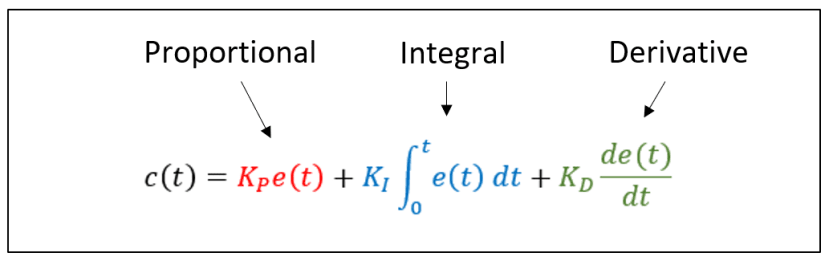
where the first term is the Proportional feedback component, the second is the Integral and the third is the Derivative. e(t) is the difference between the desired output (the set point) and the actual output. c(t) is the updated actuator control output.
A closed-loop control system utilising all three terms looks like this (Fig.1):
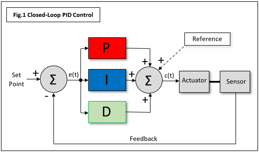
For my mobile robot example, the Actuator is a continuous-rotation servomotor and the Sensor is a reflected IR-beam unit, working with slots cut in the road wheel. Often known as a Tachometer, this type of sensor feeds back the actual wheel rotation speed data as a variable rate pulse train: the higher the speed, the faster the pulse-rate. The control program code compares this actual speed with the desired or ‘Set-point’ value and the difference is the Error input e(t) to the PID algorithm. The result is a Control output c(t) driving the motor with a value which reduces that error to zero (eventually). The three constants KP, KI and KD are usually given estimated (guessed) values initially, before being optimised on a simulation program or the actual system hardware; a process known as ‘tuning’.
PID Control in Practice
So, I bet you’re not looking forward to coding up Integration and Differentiation for real-time operation. Fortunately, there’s no need to panic, because the formula above is for Continuous Time, but this being a ‘digital’ application means that we work with sampled data measured at discrete intervals. Even better, depending upon the ‘tightness’ of the control needed, it may be possible to dispense with one or both of the I and D terms! In order to make a decision on how much of the full PID algorithm is necessary for a particular task, it’s necessary to understand the contribution of each term.
The Proportional (or Gain) Term
The P-term is essential and is the easiest to understand and implement: it’s contribution to the control signal is a proportion, set by KP, of the sensed error. Hence KP < 1. Why not make KP = 1 and cancel the whole error at once? The problem is that the electronics can turn an error signal into a revised control signal far faster than the mechanical system can react to the change. The result can be a continuous oscillation, with a motor speeding up then slowing down, above and below the set point. That’s why a proportion of the error is fed back at each interval, slowly bringing the speed to its set-point value. On the other hand, if too little is fed back, then there will be a very long wait before the required speed is reached from switch-on. So for the discrete time system:
CP(n) = KP x E(n)
Notice that the control signal reduces to zero at the same time as the error, which is somewhat self-defeating. There are two ways round this. The first is to find out what the control input needs to be for the desired set speed by running the hardware ‘open-loop’, and then adding this ‘reference’ value as a constant to the equation above. The second option is to add the Integral term described below which will zero-in on the target value automatically.
The Integral (or Reset) Term
Integrating the error signal provides a value for the accumulated error over the time interval t. In the absence of a control reference input as described above, from start-up its value should climb until it stabilises at the set-point. Normally its function is to compensate for a fixed error (offset) in the sensor measurement. If KI is too large it can cause instability though. In the discrete time system, the maths reduces to a simple addition, or more accurately, an accumulation:
A(n) = A(n-1) + E(n) where A(n) = Accumulated Error
CI(n) = KI x A(n)
The Derivative (or Rate) Term
Now we have an entirely optional component that improves performance by damping down the transient oscillation or ‘ringing’ that occurs when high values of KP and/or KI are used. This term measures the rate of change of the output and reduces the control signal as the former gets near the set-point value. With just the right value of KD, the output will not overshoot and cause over-correction. Hence we get a heavier initial control response to sudden large transients, which tapers off as the error approaches zero. The D-term can improve the response of a system to sharp changes in set-point, for example, but problems can arise due its sensitivity to noise in the feedback signal. In practice, that nasty-looking derivative term translates to a simple subtraction of the current error value from the previous one:
CD(n) = KD x (E(n-1) – E(n))
In other words, this control component is positive when the error is improving, reinforcing the effect of the P and I terms. Should the sensed output overshoot the set-point, the D term will go negative, reducing the overall control input until the error starts declining again.
The different permutations of P, I and D
The PID control algorithm does not necessarily have to be used in its entirety. Which permutation of the three terms is used for a specific application must be determined by the designer based on the characteristics of the system to be controlled. Two things need to be considered:
- How quickly the system must react to a sudden increase in the error both at initial start-up and when the set-point changes, with a steering command ,for example. This is the ‘Transient’ response.
- How closely it must track the set-point. This is the ‘Steady-State’ response.
The performance curves of some frequently used P, I, D term combinations are shown in Fig.2. The blue curve in each case is the actual output state (speed, position, temperature, etc.) relative to the desired set-point (red dotted line). Let’s assume the curve represents the speed of a motor against time t, with switch-on at t = 0.

(a) Proportional only with a fixed control reference. The reference is estimated or a value found by experiment. A large KP factor ensures a fast rise from rest, but the penalty is a lot of overshoot and ‘ringing’. An error in the reference estimate also leaves the steady-state speed somewhat less than the requested set-point value.
(b) Proportional and Integral. Keeping the same KP value, but replacing the fixed reference with the Integral term gets us to the set-point value eventually, but with even larger overshoots at first.
(c) Proportional, Integral and Derivative. In theory, with just the right value for KD something ‘magical’ happens: the ringing is almost completely damped out and steady-state is reached in a very short time.
Tuning the Loop
The maths is simple and a basic controller for a mobile robot can be run on a low-cost microcontroller board such as the Arduino. The tricky bit is selecting values for those K factors. Experience plays a big part if ‘manual’ tuning is attempted. Sometimes the system can be run ‘open-loop’ with the feedback disconnected to get an idea of its characteristics. Simulations can be run and values determined by combining experience with trial and error. Sophisticated tuning programs are available too. In practice, for small motor control like this, satisfactory results are easily obtained with a bit of guesswork and twiddling.
Next time in Part 2
For the purposes of these articles I used my trusty Parallax BoE-Bot fitted with tachometers and an Arduino-format Microchip dsPIC33 processor board providing the brain-power. Modern MCUs like the dsPIC contain special hardware for the purposes of motor control and sensing, such as ‘Output Compare’, ‘Input Capture’ and ‘Quadrature Encoder’ units. I will look at both the implementation of the PID algorithm coded in my version of the Forth language, FORTHdsPIC, and the ‘bare-metal’ assembly code drivers for the motor control and tachometer sensors.
If you're stuck for something to do, follow my posts on Twitter. I link to interesting articles on new electronics and related technologies, retweeting posts I spot about robots, space exploration and other issues.
Comments