Programming a DSP-based Digital Filter: Practical Issues

Swept-frequency response of a 62-pole digital low-pass filter with a cut-off frequency of 32.768 kHz. Note the minimal rippling in the pass- and stop-bands thanks to the Hamming window used to shape the tap-gain set. The frequency range of the sweep is from DC to 131.072 kHz, which indicates a very steep roll-off. The ‘scope is operating in X-Y mode with the output from the filter DAC on the Y-input and the ramp signal generating the frequency sweep from a function generator on the X-input. The function generator also provides the swept frequency signal to the filter ADC input.

Digital versus Analogue

My previous article talked a lot about the theoretical concept behind a digital filter; now it’s time to look at the practical aspects of actually building, or should I say programming some hardware. For the latter, I’m going to use my trusty dsPIC33E Clicker board with a plug-in ‘Click’ DAC module providing the analogue output. But first, I’ll address the question: why bother? What’s wrong with a string of Sallen-Key filters based on analogue operational amplifier technology? It all comes down to the ‘Order’ of the filter required which determines the rate at which the frequency response rolls-off beyond the so-called cut-off frequency at the high end of the spectrum, in the case of a low-pass filter (LPF). Incidentally, the terms ‘Order’ and ‘Pole’ (as in ‘First-Order’ and ‘Single-Pole’) are interchangeable for most simple filter configurations.

Using analogue technology, a 2-pole Sallen-Key Butterworth-type active filter can be realised with a single op-amp and a few capacitors and resistors. It will have a frequency roll-off of about 40dB per decade (Fig.1).

It’s often said that higher-order filters can be made easily by ‘daisy-chaining’ identical 2-pole units together. Unfortunately, it’s not that simple: each added stage not only steepens the roll-off (desirable), it also adds another 3dB to the output loss at the cut-off frequency (undesirable). It’s not good because the ‘flat’ part of the passband is reduced at the same time. Keep adding stages and eventually, the flat part of the frequency response will have disappeared. This effect is not shown in Fig.1 because the outputs have been ‘normalised’ to emphasise the difference in roll-off after the cut-off frequency at -3dB. Of course, it is possible to design a high-order analogue filter, but it can be a difficult and time-consuming exercise, particularly as the effect of ‘real’ component variations (tolerances) must be factored in. On the other hand, very high-order digital filters can be designed and emulated on a PC with suitable software. So, the first big reason for going digital with an FIR-based filter:

• A modern DSP chip with analogue I/O can replace a traditional analogue filter (or indeed, any other signal processing hardware). Prototyping just involves keystrokes rather than soldering….

Now let’s see how the marvel of digital technology enables the engineer to design filters without worrying about component tolerancing, induced noise (EMI), amplifiers turning into oscillators, ageing effects, and so on and on. Hold on, not so fast: you haven’t quite seen the last of analogue design just yet:

• Sampling theory dictates that your ADC must sample at a rate at least twice that of the highest frequency component present in the incoming analogue signal. Although techniques such as oversampling can sometimes be used to avoid frequency ‘aliasing’, a multipole analogue anti-aliasing filter may still be required. Doesn’t that render the whole digital exercise pointless….?

The answer is no. Well, probably no. In the case of signal filtering, I’ll use that overworked phrase: ‘it depends’. It depends on the filter order. If the roll-off provided by a four- or five-pole filter is sufficient, then analogue hardware based around two or three op amps should suffice. Providing the sampling frequency is well above the Nyquist limit, then a five-pole analogue circuit should be adequate as the anti-aliasing filter fronting a much more powerful, but easier to develop, digital filter. By ‘more powerful’ I mean, say, a 100-pole filter which would require 101 tap-gains to be calculated (offline), and then 101 Multiply-Accumulate operations to be performed in each sample period (real-time). Easy to program, but a little tricky finding a DSP fast enough. Not impossible though. So:

• Going digital opens up the possibility of performing complex signal processing tasks (like 100-pole filtering) that are just not feasible with analogue hardware. But, even modern DSPs may not have the bandwidth for working with high-frequency signals. As I said before: it depends…

Linear Phase

A parameter that often appears in specifications for frequency filters is a requirement for them to have a Linear Phase response, also known as constant Group Delay. Now it’s well known that electrical signals pass through a circuit at a speed somewhat less than the speed of light. When each individual frequency component of a signal moves with a speed proportional to its frequency, then the circuit, in this case a filter, is said to have linear phase. Why does it matter? For some applications it doesn’t, but for others the resulting distortion of the overall waveform shape by non-linear phase conditions can be catastrophic. Communication systems are particularly vulnerable. Take a look at Fig.2 to see why.

This shows what’s left of a square-wave after a low-pass filter has removed all frequencies bar the fundamental (in Blue) and 3^rd Harmonic (in Green). In the linear phase case, Fig.2a, the third harmonic is precisely in step with the fundamental frequency and a nice symmetrical, undistorted output (in Red) results when the two are added together. However, in Fig.2b the fundamental lags behind the third harmonic, slowed up differentially by its passage through the filter. The output waveform is now rather mangled even though the frequencies remain the same. Designing a hardware multipole filter with linear phase is no easy task. Fortunately:

• A Finite Impulse Response (FIR) digital filter will always be linear phase, providing that the tap gain set derived from the sampled impulse response is symmetrical. This remains true even if the set is truncated abruptly at each end by a rectangular window or smoothly, with say a Hamming window. Score another plus for the digital filter!

Windowing

Before addressing the issue of creating digital filter code, there is the question of how the all-important set of tap-gain values is generated. There are some direct mathematical methods, but I’ve chosen to use a technique known as ‘FIR filters by Windowing’. It actually involves using a Fast Fourier Transform (FFT) to convert the required filter’s sampled frequency response into its sampled impulse response. The latter becomes the set of tap-gains to be plugged into the real-time filter algorithm. This is relatively straightforward as far as it goes, but the snag is that an impulse response extends to infinity on each side (in theory) for a ‘brick-wall’ filter. Obviously, the response will be truncated (hence the name finite impulse response). The number of tap gains is limited by the size of the FFT, so even a 256-point FFT can provide the tap-gains for a 255-pole filter! A straight truncation of the impulse response is equivalent to the application of a rectangular window. The resulting frequency of the digital filter is less than satisfactory (Fig.3).

Both Fig.3a and Fig.3b display the frequency response of two filters with rectangular-windowed impulse responses: one with 13 taps, the other with 23. The difference in appearance between the two graphs is down to the vertical-axis scaling: [a] is linear while [b] is logarithmic (dB). So, what else do these graphs show?

• The wider the window on the impulse response, i.e. the more tap-gains used, the closer the frequency response gets to the ideal ‘brick-wall’. The ideal can never be reached, of course, because the window would have to be infinitely wide.
• There is overshoot and ‘ripple’ in both the pass- and stop-bands, which is not eliminated by increasing the number of tap-gains.
• No matter how many taps are used, the cut-off frequency f_C is always where it’s designed to be: at the half-power point as in [a], and the -3 dB point as in [b]. In other words, window size and tap-gain values only determine the filter’s roll-off and shape.

There may be applications that are not sensitive to some overshoot and ripple. In which case no further ‘processing’ of the sampled impulse response derived from the FFT is necessary. Just take as many tap gains as needed for the desired roll-off rate.

In circumstances where all that ripple is unacceptable, then replace the ‘rectangular window’ with one that smooths the edges to zero. The window functions applicable here (Hamming, Hann, etc.), are the same ones used when an FFT converts a block of time-varying data into its frequency spectrum.

The Inverse FFT

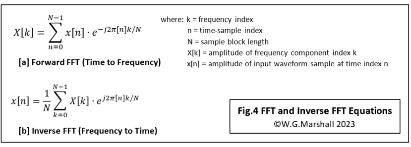
At this point, I thought I’d better clear up some potential confusion over the sort of FFT we are using here. In a lot of articles I’ve read featuring FFT applications, the ‘standard’ or forward format (Fig.4a) has been used regardless of the direction of the transformation: Time to Frequency or as here, Frequency to Time. So, strictly speaking, I should have been referring to the ‘Inverse’ FFT in these articles on digital filtering (Fig.4b). Can you spot the difference though? The 1/N scaling of the output with the Inverse is of little consequence. The important thing to note is the change of sign of the exponential; from e^-j to e^j. This corresponds to a change of sign in the expansion of the exponential from -jSinθ to +jSinθ. See a previous article of mine for more detail on the maths. It doesn’t matter which you use for the 99% of applications that involve transforming signals in one direction only. That includes, say, a design for a spectrum analyser (forward FFT) or Tap gain Generator (Inverse FFT). The FFT actually processes complex numbers with the format a + jb where a is called the ‘Real’ part, and b is the quadrature or ‘Imaginary’ component. Both applications would set the Imaginary input parts to zero because they’re working on a ‘real’ input signal. Components a and b will appear on the FFT output, but both applications are only interested in signal magnitudes derived from sqrt(a_o² + b_o²) which will be the same regardless of which FFT is used. Things only become tricky should you wish to transform the data back to the original domain, perhaps after some intermediate processing. If you want to do that, then in the case of our tap-gain generator you must first use the Inverse transform, perform the windowing on both real and imaginary outputs followed by the Forward FFT to get back to a frequency spectrum. The second FFT is not essential, but it gives you a check on what the filter’s frequency response will be.

Tricky solutions

Having said all that, there is a ‘trick’ which allows you to use two FFTs of the same type ‘back-to-back’: have the second FFT import the output Real data from the first into its Imaginary input. Similarly, route the first’s Imaginary output into the other’s Real input. In practice, this will only amount to swapping array pointers in your program code. I know of at least three other ‘tricks’, but this seems to be the most elegant.

The filter program

I discussed the basics of the real-time filter program in the previous article and you can download the full dsPIC assembler source code for a 62-pole LPF from the Downloads section below. Here are some thoughts on the code design that may prove useful when developing other real-time applications.

Unless the sampling rate is very low, the time taken for code running in the period between samples is critical. No time can be wasted in loops waiting for something to happen; in the digital filter case no looping until the ADC has acquired the next sample or waiting for the DAC to settle. It’s best to eliminate any test-and-branch loops including those that determine the end of the process cycle and trigger the resetting of counters and buffer pointers. My digital filter code loop is contained entirely within the Interrupt Service Routine (ISR) for the dsPIC’s Timer 1 – the sampling clock. The reset/power-up initialisation code is of course only executed once, leaving a single ‘branch-to self’ instruction acting as the base program periodically interrupted by the sampling Timer 1. In order to monitor just how long one cycle of the filter code actually takes to run, I inserted an instruction to set port bit B15 at the beginning, and a clear bit B15 instruction at the end just before the return from interrupt instruction. On a ‘scope attached to the port pin, a stable pulse train should be visible with the time between rising edges corresponding to the sampling period. The length of the ‘high’ interval represents the cycle-time for the filter. The ‘low’ interval tells you how much time is available for base program execution. Now that’s important because building and programming a DSP system just to perform a low-pass filter function makes little sense. Unless a near-brick-wall response requiring many poles is essential for subsequent processing by a further DSP/MCU. A more moderate (fewer poles) filter might leave sufficient time for that other processing to be performed by the same DSP chip.

Optimal use of hardware

DSP chips have special instructions like the dsPIC’s MAC which fetches operands, performs a multiply-and-add to a 40-bit accumulator and adjusts the index registers to fetch the next operands. All in one machine cycle.

Sometimes overlooked are the instructions like REPEAT and DO, which work with special hardware counters and registers, enabling ‘zero-overhead’ loop control. See how the use of REPEAT and MAC reduces the core filter loop to just four single-cycle instructions.

The ADC sample capture routine at the start of the ISR would normally execute a start conversion instruction and the enter a loop waiting for the DONE flag to become set before reading the data. In order to avoid using a test-and-branch loop, I’ve used the REPEAT instruction to execute a number of do-nothing NOPs instead before proceeding. Getting rid of the conditional branch can eliminate timing variations being introduced by the BRA instruction which requires one cycle to execute if no branch takes place, but four if it does. Not important here, but it’s something which might cause timing ‘jitter’ in other applications.

The use of REPEAT to optimise the core filter code has already been mentioned, but that’s only possible thanks to a further piece of internal special hardware. It enables a special addressing mode allowing two zero-overhead Circular Buffers to be operated. Each buffer is a block of RAM the same length as the number of tap-gains. One contains the tap-gain list itself and is read-only. The other is the filter data buffer with new data being introduced at the low-address end, and output samples taken from the top. With the extra hardware, no instructions are necessary to detect when index pointers reach the top, and to reset them to their new start positions after every filter cycle. That sort of saving makes a big difference to execution times.

The DAC is external to the DSP and data is sent to it via a serial SPI bus. A large amount of time could be wasted here if the normal convention of waiting for transmitted data to be received before sending more. That protocol is unnecessary here because single data-word transmissions are always separated by relatively lengthy intervals of idling. The SPI bus is used in preference to UART or I2C because it’s very fast; in this case, operating at 17.5 Mbits/sec with no protocol overhead.

Finally

These two articles represent a far from exhaustive treatment of the topic, but if you’ve not tried programming a real-time system working with high-speed signals, I hope I’ve demonstrated that there’s no room for sloppy code. It must be tight to accommodate the desired algorithm at the specified sampling rate, and it must exhibit consistent timing so that the output doesn’t ‘jitter around’ and upset the systems downstream. Incidentally, the program to create the tap-gains can be written on any old computer, preferably in a language with floating-point maths and trig functions. Many language implementations have maths libraries containing even higher-level functions such as the FFT and its Inverse. I didn’t bother to write a tap-gain generator for this project. I already possessed one, written in 1986 for a BBC Model B microcomputer. It works a treat on my PC via the excellent BeebEm emulator!

If you're stuck for something to do, follow my posts on Twitter. I link to interesting articles on new electronics and related technologies, retweeting posts I spot about robots, space exploration and other issues. To see my back catalogue of recent DesignSpark blog posts type “billsblog” into the Search box above.