Frequency Analysis for Embedded Microcontrollers, Part 5

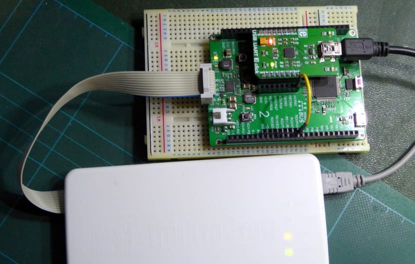
MikroElektronika Clicker 2 board (170-8233) with a Mikroprog programming/debug module attached to the ICSP connector. A UART-USB bridge Click module (184-0913) is plugged in for PC terminal communication. The yellow wire links the programmed test signal generator output to the ADC input.

A change of platform

The development kit I’ve used so far in this series has been the dual-core dsPIC33CH-based Curiosity board (187-6209) . The aim was, and still is, to create an FFT routine for my FORTHdsPIC real-time embedded programming system. FFT code will run on the fast (100 MHz) Slave processor called by user Forth code running on the Master. However, I’ve since got a bit distracted by the idea of creating a pocket-sized spectrum analyser based on a Mikromedia dsPIC33E board. Regular readers of my blog posts in recent years will have become familiar with MikroElektronika’s range of development boards and ‘Click’ expansion modules. Their dsPIC33E Clicker 2 processor board has been the host for my FORTHdsPIC code for some time now: more information is available on the Project page. The Clicker 2 is Arduino-sized and features a Microchip dsPIC33EP512MU810 chip with two Click module sockets. The Mikromedia board has the same format and uses the same chip, but the two Click sockets are replaced by a 2.8in 320 x 240 pixel TFT touchscreen. Unfortunately, the chip shortage is still with us and I’m having some difficulty tracking one down. Until I do, development work can continue using the Clicker 2 platform instead.

Analogue data acquisition

To aid debugging of the FFT code, the 256-word input buffer was programmed with an ‘ideal’ set of data samples. They represented a 50:50 duty-cycle pulse train, also known as a ‘square wave’. An integer number of cycles in the buffer ensured a spectrum consisting of a DC level, a fundamental frequency set by the number of cycles, followed by odd harmonics only, third, fifth, and so on. A non-integer number of cycles was used to demonstrate spectral leakage effects. See Part 3 and Part 4 for the results.

The next step was to capture ‘real’ waveforms in real-time by using an Analogue to Digital Converter (ADC) conveniently present on the dsPIC chip itself. Of course, I now needed an analogue signal to sample and process. So, not having a suitable signal generator to hand, I set up one of the chip’s Output Compare modules as a PWM generator. Any frequency may be set under program control, as can the duty-cycle of the pulses. The only extra ‘hardware’ is the single yellow wire in the heading photo linking a PWM output to an ADC input channel, AN2. Once this is set operating, it runs asynchronously with ADC sampling.

Design considerations

One of the big advantages of digital, as opposed to analogue signal processing, is that changes to parameters such as frequency bandwidth only require changes to numbers, not physical components.

Sampling rate selection

The first parameter to be decided upon is the Sampling Rate (f_S) for the system. We know that the lowest possible value must be at least twice the highest frequency component present in the input signal: the so-called Nyquist-Shannon frequency. I wanted my audio spectrum analyser to be able to handle frequencies up to 250 kHz, for which a sampling rate of 500 kHz is needed. Audio frequencies are normally considered to be below 20 kHz, so why the massive ‘over-sampling’? The ability to resolve high out-of-band frequency components is necessary to reduce the complexity of the analogue anti-aliasing filter that sits between the analyser input and the processor chip’s ADC input pin. For more details on this subject, read this article. The actual rate used here is 524288 Hz, a nice round ‘binary’ number (80000h) to make calculations easier – remember the FFT only works with binary quantities such as 256 samples in a block.

A further aspect of sampling rate selection is accuracy. The sampling clock must be very accurate and stable if you expect the output from this frequency analyser to be meaningful. The sampling clock signal is derived from the dsPIC’s master oscillator running with an external 8 MHz crystal in XT mode. This crystal needs to be of high quality, and ideally contained within a temperature-controlled oven for maximum stability. A bit over-the-top perhaps for this project; in any case the Clicker 2 board comes fitted with a simple crystal which should prove adequate. The crystal frequency is multiplied using a built-in phase-locked loop (PLL) circuit to generate a nominal processor clock of 140 MHz. The user has access to the PLL feedback register which means there is scope for tweaking the clock frequency to compensate for crystal oscillator inaccuracy. Timer 1 is programmed to divide down the master clock to the desired sampling rate.

Sampling block size (N)

The nature of the FFT algorithm limits sampling block sizes to binary quantities such as 256, 1024, 2048 and so on. As we have seen, this restriction is the payback for the massive increase in speed over the basic DFT. As a starting point, I went with the block size of 256 that was used for the earlier program development. This parameter determines the frequency resolution of the output spectrum for a given sampling frequency:

Resolution or Spectral Line Separation f_R = f_S/N Hz

So, for my system: f_R = 524288/256 = 2048 Hz. That means that the only frequencies appearing cleanly, with no spectral leakage, will be 2048 Hz, 4096 Hz, 8192 Hz, and so on, up to 262144 Hz. Not good, is it? But here are some results starting with my favourite test waveform: a square wave that fills the block buffer with an integer number of cycles.

Figure 1 above shows the output from the FFT when the input is an 8192 Hz square wave – real sampled data this time via an ADC, but I’ll talk about that later. The frequency spectrum is clean and there are no spectral leakage artefacts. That’s because 8192 is an integer multiple of 2048 placing the fundamental at bin 4, the third harmonic at bin 12, and so on. An absence of ‘even’ harmonics is in evidence, thanks to the 50:50 mark/space ratio of the pulse train.

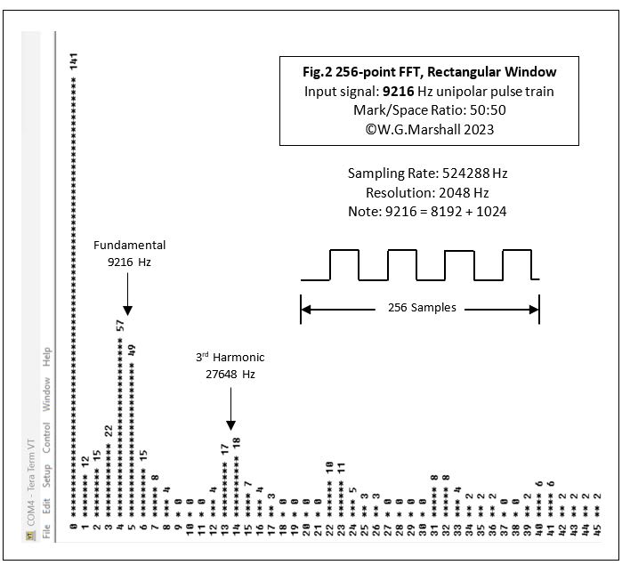
Figure 2 shows the output when the frequency is increased from 8192 to 9216 Hz. Despite all the leakage, the positions of the ‘real’ frequencies can be deduced as lying halfway between bins 4 and 5, 13 and 14, and so on. The absence of even harmonics is still in evidence because the mark/space ratio hasn’t changed.

Keeping the pulse frequency at 9216 Hz but changing the mark/space ratio to 25:75 leads to the spectrum of Figure 3. The even harmonics (2^nd, 4^th, 6^th, etc) have now appeared as clean single lines as they are all ‘bin’ frequencies. For example:

f_R = 2048 Hz

Fundamental = 4.5 x f_R = 9162 Hz

2^nd harmonic = 2 x fundamental = 9 x f_R = 18432 Hz

4^th harmonic = 4 x fundamental = 18 x f_R = 34816 Hz

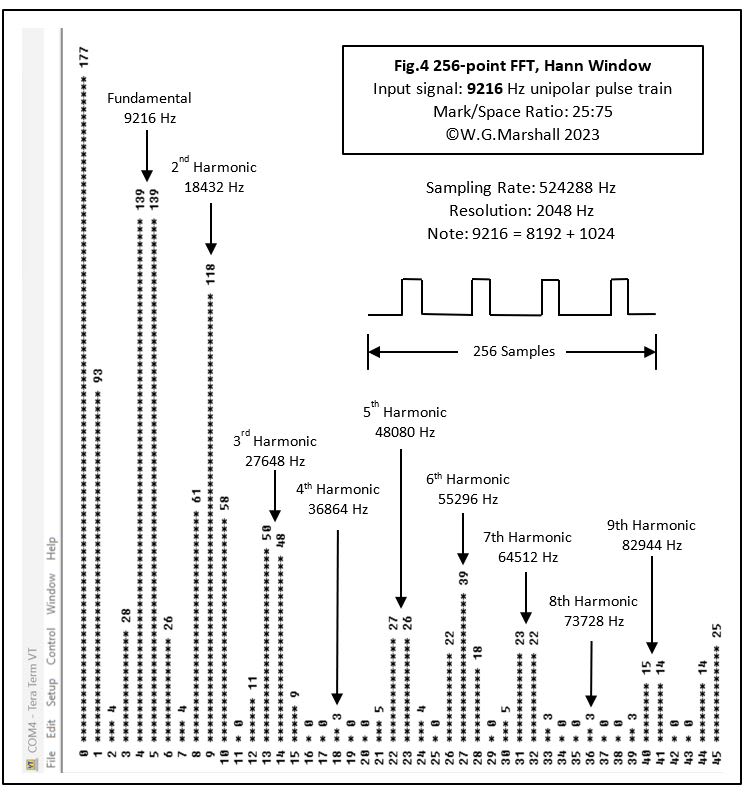
Finally, Figure 4 shows the effect of pre-processing the sample block with a Hann window. Notice how most of the low-level spectral leakage has been suppressed. The ‘sidebands’ around the DC offset and the even harmonics are an artifact of the windowing, but in general, the resulting spectrum is easier to interpret than that of Figure 3.

Better resolution

Two things can be done to improve the resolution:

1. Increase the block length or
2. Reduce the sampling rate.

I decided to increase the block length to 1024 samples which means using a 1024-point FFT. The resolution is increased to 512 Hz, better but still not great, especially when sampling audio signals. The FFT will obviously take longer to compute too. Reducing the sampling rate will improve resolution, but at a cost of reduced input signal bandwidth. But what about giving the analyser a range switch controlling the sampling clock and, most importantly, the cut-off frequency of the anti-aliasing filter? So, for example, you could have a low-range setting of up to 512 Hz for looking at mains-borne interference signals:

Max input frequency = 512 Hz, so f_S = 1024 Hz minimum

If N =1024 then f_R = 1024/1024 = 1 Hz

Another useful range would be 20480 Hz for audio work which would then have a resolution of 40 Hz with N = 1024 and f_S = 40960 Hz.

A design problem arises with operation just on the Nyquist limit: the anti-aliasing filter must have a steep roll-off. A compromise design may be needed if the analogue filter is not to get unduly complex.

Real-time operation

The test program (see Download section), after initialisation, grabs a block of data from the analogue input at the sampling rate (524288 Hz). This 256-word data block is then converted to 256 frequency samples by the FFT. Finally, the results are sent via a serial COM port for display on a PC screen by Tera Term software. The program then halts and processes another block when any keyboard key is pressed. Not exactly a real-time display, but good enough for testing! It’s important to note a whole data block is captured before the FFT executes. Ideally, for true real-time operation, the FFT code should execute while the next block is captured. This may be possible if data capture by the ADC can be automated with DMA. Something to look at later. In the meantime, the gaps when no data is being captured don’t matter if all we’re doing is displaying the results on an LCD. The ‘update’ period will still be in the milliseconds range and barely noticeable to the viewer, if at all.

Next time in Part 6

The output display part of this saga may well be delayed for some time if the chip shortage prevents me from getting my hands on a Mikromedia board! In the meantime, I'll be adding code to provide a logarithmic output in decibels (dB); a task not made any easier by working with integer rather than floating-point arithmetic.

If you're stuck for something to do, follow my posts on Twitter. I link to interesting articles on new electronics and related technologies, retweeting posts I spot about robots, space exploration and other issues. To see my back catalogue of recent DesignSpark blog posts type “billsblog” into the Search box above.