RF Communications and the Internet of Things - Part 5
Follow article
 Dave from DesignSpark
How do you feel about this article? Help us to provide better content for you.
Dave from DesignSpark
Thank you! Your feedback has been received.
Dave from DesignSpark
There was a problem submitting your feedback, please try again later.
Dave from DesignSpark
What do you think of this article?
This fifth and final part of my wander through the world of wireless digital communication covers relatively long-range working. By ‘long-range’ I mean up to about 20km as opposed to the really, really long distances described in Part 2. Indoor stuff was covered in Part 4. After a comparison of (currently) the two main players in this area, LoRaWAN and SIGFOX, I finish with a guide to some of the most important parameters to understand on an RF module datasheet. Then you can get that toaster sending important breakfast data to the Cloud. If you feel the need.
Long-Range IoT
As a general rule we work with the sub-1GHz carrier frequency bands once communication moves outdoors: 868MHz ISM band (Europe) and 915MHz ISM band (USA). Transceiver modules for these bands have been around for years but were really only used in specialised industrial or commercial applications. In most cases the user would have to write their own custom protocol to suit a particular application. Then came the Internet of Things. Actually, Machine-to-Machine (M2M) networks existed before the IoT, but usually in the form of cable links. Now the push is on to replace all that cable in factories sites with much more flexible wireless network operation forming the Industrial Internet of Things (IIoT). Whole cities/regions are getting networked too, leading to the establishment of a low data rate Internet of Things separate from the current high-speed broadband cellular networks. Two different approaches both in technology and business model have emerged in a race to set up this worldwide LPWAN network: LoRaWAN and SIGFOX.
LoRaWAN™ Networks
I described the hardware behind LoRa, the Chirp Spread Spectrum technology proprietary to Semtech, in Part 3. The LoRa Alliance has produced an open specification for a network protocol called LoRaWAN and anybody can make a module or gateway based upon it. The only catch is that the radio chips will only be available from Semtech or other licensed manufacturers. This open-source aspect of LoRaWAN has led to some crowdsourced networks being set up such as The Things Network. Successful ‘Things Networks’ have been set up in Amsterdam and Reading in the UK.
Topology and Operation
A simple LoRaWAN network has a Star topology with a number of ‘End-Devices’ or ‘nodes’ linked to a Gateway. The nodes cannot communicate with each other directly as with a Mesh-based system and this saves power as there is no message ‘forwarding’ requirement. Expanding the network consists of creating more Stars and linking the Gateways together to form a Star-to-Star topology. Each Gateway connects to the high-speed Internet - the ‘Cloud’ - and acts as a ‘concentrator’ for thousands of LoRaWAN nodes. It should be apparent at this point that there is a potential traffic problem if all the nodes try to talk to a Gateway at the same time. Chaos is avoided thanks to the network Cloud Server managing the data rate and RF output for each node individually. The LoRa protocol provides multiple variable-bandwidth channels with variable Spreading Factors and data rates. A powerful feature of Chirp spread spectrum modulation is that signals with different Spreading Factors can co-exist in the same channel. This of course means that a Gateway will contain multiple modems, each ‘tuned’ to a different Spreading Factor. This complexity does however permit the end-device to be mobile.
Classification of End-Devices
Fortunately the nature of IoT sensor operation means that a node only sends small amounts of data at widely spaced intervals and seldom needs to receive any. The European regulations for the main RF band used by LoRa (865-868MHz) stipulate a maximum transmission ‘Duty-Cycle’ of 1%. In other words an individual node may only switch its transmitter on for up to 36 seconds in an hour. The LoRaWAN specification defines three classes of node, A, B and C depending on how attentive it is to transmissions from the Gateway:
Class A: Uses the least power as it only listens to the Gateway during two short time windows after it has transmitted some data. It’s ideal for battery-powered sensors.
Class B: Operates as for Class A, but will also open scheduled receive windows in response to a beacon signal from the Gateway. This class is ideal for battery-powered actuators, but consumes a bit more power than Class A.
Class C: These devices tend to be mains-powered and are always listening except when transmitting.
Summary
LoRaWAN has been designed for the classic Internet of Things network concept where remote, low-power sensors send occasional small packets of data to an application in the Internet Cloud. Under the control of a central server, it uses adaptive data rates (ADR) to ensure reliable communication with many thousands of battery or energy-harvesting powered end-devices. The communication link is symmetrically bi-directional so end-devices can be sensors, actuators or both. Networks can be set up by individuals or institutions who purchase a Gateway, install it on their own premises and provide the Internet link via an existing router. Networks across Reading and Glasgow have been set up in this way. A co-existence problem with other communication systems operating in the same band may develop because of its wide-band format: it will appear as increased channel noise by ‘raising the noise floor’ for narrowband protocols such as those used in:
SIGFOX™ Networks
SIGFOX wireless technology is based upon tried and tested modulation schemes and achieves similar receiver sensitivities and range performance to LoRa by using Ultra-Narrowband (UNB) channels in contrast to LoRa’s wideband spread-spectrum technique. The business model is also different: end-devices must be SIGFOX-certified and operate over SIGFOX or SIGFOX-affiliated networks.
Topology and Operation
SIGFOX operates rather like the existing cellular telephone networks but with its own base-station towers. The base station hardware is thus considerably more expensive than a LoRaWAN Gateway. The narrow channel bandwidth allows for a lot of channels within the chosen ISM frequency band with BPSK modulation and frequency hopping (FHSS). The downside of a narrow channel is the severely reduced data rate: 100bps uplink with a message payload of 12 bytes. Further, the 1% duty-cycle restriction on the 868MHz band restricts you to fewer than 140 messages/Thing/day. A downlink is also provided operating on a slightly different carrier frequency at 600bps with GFSK modulation. Hence simultaneous bi-directional operation (Full-Duplex) is possible. Realistically, Sigfox is aimed at simple one-way communication applications such as meter-reading and basic alarm systems. There is no ‘message received’ acknowledgement feature of ‘Listen Before Transmit (LBT)’ to avoid collisions so messages are typically sent three times – just to make sure.
Fortunately, the upside to ultra-narrowband operation is drastically improved receiver sensitivity. For those with some interest as to how this works should take a look at Appendix 2 below.
Summary
Like LoRaWAN, SIGFOX was developed for the Internet of Things providing the essential link for large numbers of very-low power sensors occasionally sending small amounts of data slowly to the very fast, ‘big-data’ domain of the Cloud. A fierce debate has been running about the relative merits/demerits of the different approaches taken by SIGFOX and LoRaWAN. The argument comes down to which system works better in the real, crowded world: ultra-narrowband lowering the noise floor and thus increasing Receiver Sensitivity; or wide-band Spread-Spectrum utilising huge amounts of ‘redundancy’ extracting signals from below a much higher noise floor. The latter has Processing Gain from all the redundancy which leads to an improvement in Receiver Sensitivity.
Read this Texas Instruments paper on narrowband communication. It could be argued that the author is somewhat biased as TI is pushing an existing range of their narrowband transceiver chips suitable for use with SIGFOX, whereas SemTech has the sole rights to the LoRa Chirp Spread Spectrum technology.
The Bottom Line
No matter what the technical arguments, the bottom line is: how easy is it to ‘get connected’ with the Internet of Things using either of these two systems?’ If you want to set up your own private network, or get involved with one of the Things Network projects then LoRaWAN is the one. On the other hand, going with SIGFOX cuts out all the hassle of generating a new network, by using an existing Service Provider. Commercial LoRaWAN networks are being set up too, and the same advice applies to both: check that coverage is available in your geographical area!
Actual user experience is a little thin on the ground at the moment, but as networks of both flavours are set up it may soon become apparent if there is going to be a ‘winner’. Or maybe one of the following technologies will grab the market.
WiFi for Long-Range IP-Based Networks - HaLow

The average home already has a WiFi communication network connecting printers to computer devices, and devices to each other and the Internet. While in principle WiFi protocol IEEE 802.11b/g/n could be used for IoT purposes, it is not suited to the IoT’s characteristics of low-power, low-data rate and potentially large number of connected devices. The range is also restricted because of the 2.4GHz operating frequency. These issues have been addressed with the announcement of the IEEE 802.11ah standard, which the Wi-Fi Alliance have incorporated in a protocol called HaLow. Like Bluetooth BLE, HaLow is designed to work with typical IoT devices, but the extra step has been taken to shift the carrier frequency into the sub-1GHz band making it suitable for longer-range, outdoor applications. Because HaLow is IP-based it has the potential to provide seamless communication between devices and ‘the Cloud’ eliminating the need for much bridge and gateway hardware. Watch this space.
IoT over Cellular Networks – LTE Cat-M1 and LTE Cat-M2 (NB-IoT)
The Third Generation Partnership Project (3GPP) is a technical body that develops standards for cellular phone communications. Recently the mobile operators with big investments in the cellular network hardware decided they wanted a piece of the IoT action and are now pushing the new 3GPP standards LTE Cat-M1 and LTE Cat-M2. The latter is also known as Narrowband-IoT or NB-IoT. Cat-M1 is a reduced bandwidth/data rate/power protocol which can be deployed on current cellular networks. Cat-M2 is even more reduced but isn’t compatible with current LTE networks and would require chunks of GSM bandwidth to be allocated to it. Neither has been deployed yet and it remains to be seen whether the operators will accept the allocation of LTE bandwidth to Cat-M2 for IoT or Machine-Type Communication (MTC). In the meantime this paper provides a useful summary of the various options that are, and may become available in the near future.
That’s All Folks
Of course, that’s not all there is to it. The topic is constantly evolving with technical improvements and new applications rendering these posts out-of-date within months – except for the basic principles; they will always remain the same. At the time of writing the IoT still faces two big questions: do we really need it and will it survive criminal attack? A possible affirmative answer to the first came from JPL/NASA recently. As to security, it's no secret that there are unresolved problems regarding unauthorised access to sensitive data on the Internet. At one end of the scale there is a vast amount of personal data pouring into the Cloud from 'Fitness Bands'. At the other, you have industrial plants with heavy machinery controlled via wireless links - the so-called Industrial Internet of Things (IIoT). It doesn't require a clever hacker to wreak havoc; just a a disgruntled employee or competitor with a powerful wideband jammer outside the perimeter fence. Sooner or later someone is going to cut costs by running a power station nuclear reactor wirelessly. Makes me shudder to think about it.
Appendix 1. Datasheets and Practical Aspects
Watching out for manufacturers’ ‘specmanship’ on datasheets is a skill engineers of any persuasion will learn pretty quickly. You know the sort of thing: a MOSFET has a headline current rating of 100A for example. Further down the datasheet in a complicated table is the information that this rating applies only when a half-acre heatsink with forced-draught cooling is employed, otherwise the maximum is 20mA. Alright, that’s an exaggeration, but not as much as you might think. Wireless radio modules often suffer from the omission of qualifying conditions and it’s easy to be misled. When developing an RF wireless communication (radio) link, the most basic calculation required is the Link Budget (see Part 1.). You will need to obtain the maximum range and the likely data rate to make an initial selection of possible technologies. Then start looking at some datasheets and watch out for ‘weasel’ performance claims.
- Transmitter Power Output. Normally the maximum power emitted from a half-wave dipole antenna is quoted, known as the Effective Radiated Power (ERP). Usually this value will be defined by regulation limits – but check as it may vary between regions. Sometimes the Effective Isotropic Radiated Power (EIRP) is specified which assumes an ideal point-source antenna. This isotropic radiator radiates power evenly in all directions and is only a theoretical concept however, (see Part 1). Real antennas don't have this spherical radiation pattern: a vertical dipole's pattern is torus-shaped, boosting the signal power in a horizontal plane at the expense of the vertical. Hence if the ERP value is specified it includes a +2.19dBi boost in the favoured direction for a half-wave dipole, or +5.19dBi for the more familiar stubby quarter-wave monopole. The units of antenna gain are dBi to indicate that it is relative to the isotropic EIRP value. Most modules/chips are programmable for output power so meeting regulations should not be a problem.
- Receiver Sensitivity. This is the parameter that suffers most from ‘weaseling’. The best (lowest) possible figure is always quoted in the headline specification and if you’re lucky a table on page 94 will supply the conditions for which it is true. In all cases the best sensitivity is only available at the slowest data rate. This neatly leads on to the next parameter:
- OTA Data Rate. OTA means ‘Over-the-Air’ and refers unsurprisingly to the data rate of the RF channel. The OTA part is often omitted on datasheets and so there can be confusion with the Host Data Rate which applies to the serial link with a host microcontroller. Headline OTA rates are always the maximum possible which corresponds to the poorest value for receiver sensitivity and thus the shortest range.
- Range. You should be getting the idea by now. When range is quoted, naturally it will be the longest possible. An important condition to achieve this performance is rarely mentioned in the headline: the transmitter and receiver antennas must be within ‘line of sight’ of each other. In other words if you are standing beside the transmitter, you must be able to see the receiver (You might need binoculars). Any obstructions like buildings for example, will drastically reduce the effective range in a random, unpredictable manner. The Free Space Loss factor (see Part 1) used in the calculation of a link budget does not include the effect of obstacles such as buildings.
- Link Budget. The general view is that the link budget is an equation which links Transmitter Power, Antenna Gain(s), Free Space Loss and Receiver Sensitivity. Strictly, the last should be Received Power, but we might as well include the Link Margin to give us a minimum received power that results in successful demodulation. Given four of these, one unknown can be calculated. Sometimes you will come across a parameter on a datasheet called Link Budget. This is usually given by: Max Rx Sensitivity - Max Tx Power in dB ignoring antenna gains. For example:
Link Budget = -120 - 10 = -130 dB which gives you a worst case for channel losses.
Boosting the Range
Sometimes you will come across third-party ‘tests’ of a particular RF module that shows miraculous range performance. Check the antenna(s) used in the test. The most obvious range-booster is a high-gain transmitter antenna to replace the simple monopole or dipole item usually supplied. Tempting, but you will fall foul of the regulations. In most regions at 868MHz, transmitter antenna gain of up to +6dB is permissible on top of the regulation maximum EIRP. Thereafter increases in antenna gain must be matched by a corresponding drop in EIRP. This means that you are just about on the limit with the standard quarter-wave monopole. So is there any point in exchanging radiated power for antenna gain? Yes, actually. By performing this swap you may not be extending the range, but you will be making it more focussed. If all that’s needed is a fixed link between two points then broadcasting energy in all directions is a waste of power. A tight beam formed by a high-gain, highly-directional Yagi array or parabolic dish will do the job nicely (see Part 2 for an extreme example). Of course this does not apply in a LoRaWAN or SIGFOX network say, where nodes and Gateways need to be as omnidirectional as possible.
Extending range by using a high-gain receiver antenna causes no conflict with regulations and its use often accounts for the great range achieved by tiny RF modules in published tests. A bonus from reducing the coverage of a receiver to a beam is a reduction in the interference from unwanted transmissions nearby.
Appendix 2. Calculating Receiver Sensitivity
A key factor of Sensitivity is the receiver bandwidth which influences how much of the channel thermal noise gets to the demodulator circuits. The wider the bandwidth, the greater the amount of noise getting through and hence the worse the sensitivity. Or to use an old RF engineer’s adage: ‘the more you open the window, the more muck flies in’. Only they didn’t say ‘muck’.
Lowering the Noise Floor
This thermal ‘noise floor’ parameter is derived from the expression:
Noise Floor = 10log10(kT) + 30 + 10log10B dBm
where k = Boltzmann’s Constant , 1.38 x 10⁻²³ W/HzK, T = Temperature in K, B = Receiver Noise Bandwidth
Most designers assume room temperature operation so T = 290K. The +30 number converts the power from dBW to dBm, giving us:
Noise Floor = -174 + 10log10B dBm
So for example a 1MHz channel yields a noise floor = -114dBm. Narrowing the bandwidth to 12.5kHz drops the noise floor to -133dBm.
The value for Receiver Sensitivity is arrived at by adding the receiver circuit’s own electronic noise, the Noise Figure (NF) and the Carrier/Noise Ratio needed for successful demodulation – both in dBs. In a digital communication system, the parameter C/N is defined in ‘digital’ terms:
C/N = (EB/NO) x (R/B) = 10log10(EB/NO) + 10log10(R/B) dB
where EB = Signal Energy per Bit, NO = Noise Power per Hz and R = Bit Rate, B = Noise Bandwidth
What Constitutes ‘Successful Demodulation’?
You may ask. It’s a bit subjective in the analogue world, but with digital it can be quantified in terms of the proportion of bit-errors in a transmission of a given length. Most datasheets will quote Receiver Sensitivity based on a maximum of 1 bit in 1000 being incorrect. Or using the accepted terminology: a Bit Error Rate (BER) of 0.1%. I’ve not come across much weaselling on datasheets here, but many omit to mention the BER used in the calculation. Having got a figure for BER and knowing the modulation technique employed (BPSK, FSK, etc.) the value for EB/NO can be read straight off the published BER graph (see Part 2). So now:
Receiver Sensitivity = Noise Floor + NF + C/N dBm
Seasoned designers will quibble about the vagueness of the term ‘Bandwidth’. In this case its full name should be: ‘Equivalent Noise Bandwidth’. It isn’t quite the same as the channel bandwidth and requires further calculation to be strictly accurate. This article from the High Frequency Electronics website will tell you all you need to know.
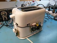
Heading picture: Toaster with Raspberry Pi at Hacklab Turku. Made by Juuso. Hannu-Makarainen
Part 1. IoT Communication: Decibels, Free State Losses, Link Budgets and CubeSats
Part 2. IoT Communication: Noise, Interference and Communicating with Pluto
Part 3. IoT Communication: Modulation, Coexistence, Spread-Spectrum and Chirps
Part 4. IoT Communication: Regulations and Short-Range IoT
Part 5. IoT Communication: Long-Range IoT, Datasheet Hype and Future Technologies
If you're stuck for something to do, follow my posts on Twitter. I link to interesting articles on new electronics and related technologies, retweeting posts I spot about robots, space exploration and other issues.