Getting The Most Out Of Your Oscilloscope: Cursors and Parameters

Oscilloscopes give us a wealth of tools with which to view, measure, and analyze the performance of a circuit. Broadly speaking, two classes of such tools are cursors and parameter measurements. Taken on their own, both classes afford the user a great deal of capability. Put them together, though, and you can really start to gain deep insights into what's going on with a waveform.

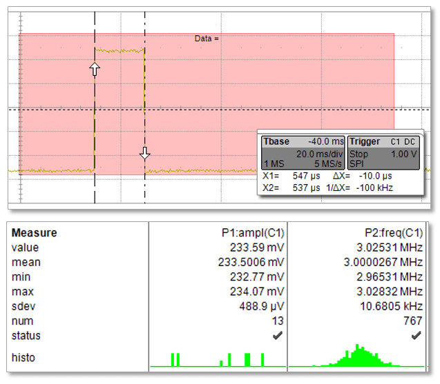
Figure_115_d01a8c53223cbae0ef610a457d2cc60144ce17c0.png Figure 1: Cursors (top) and parameter measurements (bottom) are both powerful tools in their own right

Once you've acquired a waveform, you can quickly apply some cursors (Figure 1, top) to help with measurements. There are three basic types:

- Voltage (Vertical) cursors are dashed lines that you move vertically on the grid to measure the voltage levels of a signal. When used on a FFT waveform, dBV values are measured.
- Time (Horizontal) cursors are dashed lines that you move horizontally on the grid to measure the time values of a signal. When used on a FFT waveform, frequency values are measured.
- Track (Horizontal) cursors are cross-hairs that you move horizontally along any channel waveform. Place them at desired locations along the time axis to read the signal’s voltage levels at the selected times.

While cursors are extremely useful, they remain manual in terms of how they're deployed. Parameter measurements, however, are automatic, highly accurate, and perhaps most importantly, they can be gated, allowing you to define where in the waveform you're taking the measurements. Instead of measuring the mean value for a parameter over the entire waveform, you can define specific parts of the waveform and limit the measurement to that portion.

Figure 2: Parameter measurements are displayed in a table along with statistics and histicons

Parameter measurements are displayed in tabular form (Figure 2); this example shows eight parameters being measured on the signal but you can have as many as 12 at once with Teledyne LeCroy's 12-bit, 8-channel oscilloscopes. The dialogue box at the bottom in Figure 2 is open to tab P3, which in this case is frequency. Meanwhile, with each acquisition, all of the parameters are being measured and compiled in the statistics shown in the parameter table.

Figure 3: Parameters can be viewed all at once or by categories, and with or without descriptions

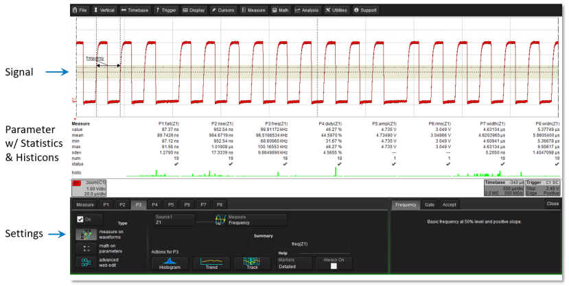
There's quite a large selection of parameter measurements, depending on the options installed in your Teledyne LeCroy oscilloscope (Figure 3). You can view the entire list by selecting All Measure when you're choosing a parameter, or you can view them by various categories. If you don't want or need to see the parameter descriptions, there's a button to the bottom left of the dialogue box that lets you view them as icons. This lets you see more of them at a given time.

Let's take a closer look at parameter statistics for a moment. In the measurement control dialogue box, you can find options for turning on statistics and histicons. The parameter statistics, which are compiled for all instances of a measurement, include the last measured value, the mean of all measurements, minimum and maximum values, standard deviation, and the number of measurements.

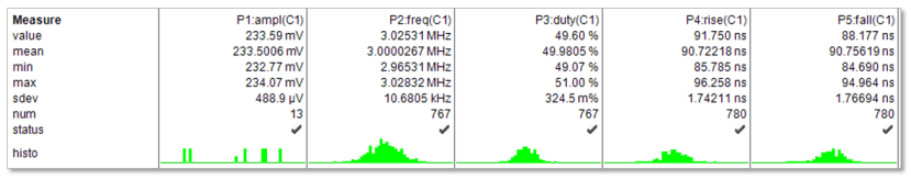
Figure 4: A parameter table's statistics can reveal interesting information about the waveform being measured

In the example statistics table of Figure 4, we can see that 13 amplitude measurements were taken, which says that we acquired 13 waveforms. Note that there are 767 frequency and duty-cycle measurements, but 780 rise- and fall-time measurements, which might be an interesting detail. At the bottom of each parameter, the measurement list is the corresponding histicon, which gives you a thumbnail graphical representation of how the statistical data is changing over time.

What histicons are actually showing you is the distribution of the measurements. They show you graphically whether the measurements are grouped around a mean value and whether there are any outliers among them. If so, then you probably want to move into troubleshooting mode.

Figure 5: square wave acquisition

Figure 5 is a screen capture of a square wave acquisition. Let's say we want to take a better look at the statistics for P4, the pulse-width measurement of the Ch1 waveform. Instead of using the histicon for insight, we can open a Math channel and turn to a live histogram of the statistics. It's the same data as in the histicon, but now you can apply cursors to the different bins of the histogram. We can see from the statistics table that we've taken some 9000 pulse-width measurements from 363 acquisitions with a mean value of about 197 µs. But we also note that there's been a glitch of 165 ns. Cursors will help us determine from the histogram how many glitch pulses have occurred.

We'll continue looking at ways to get more out of your oscilloscope in upcoming posts.