PYTHON – Let the „Monty-language” enter Automation: Part 3

If you are still following this series, you have hopefully successfully built your hardware setup from part 1 and survived an installation marathon of part 2. Until now, we have not written a single byte of Python code. It's time to change this.

Because I like to use the interactive possibilities of testing and debugging, I use the Python IDE “IDLE” which comes with the RevPi. We use the VNC connection to start it from the RevPi desktop:

Click on the red raspberry, then open “Programming” and click on Python 3 (IDLE). If you are interested in the discussion about using Python 2 or Python 3, you are welcome to dive into this “religious war” by googling and surfing on the internet. For now, simply follow me using Python 3 and I guarantee you will end up happy ;-)

If you have done so, a window with the “Python Shell” has opened:

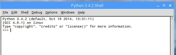
The prompt “>>>” indicates, that the system is waiting to execute a Python expression. Python is an interpreted language, and nothing is compiled in advanced. Everything you type is executed. So type in the expression “4+5 <enter>, and you get the system’s answer “9”:

>>> 4+5

9

>>> 

I frequently use this possibility to execute a line of code when I’m not sure about the correct syntax or the type of result. E.g. typing 2^8 to get 2 to the power of 8 you get:

>>> 2^10

10

Showing you that the syntax is wrong whereas 2**8 results in what you want:

>>> 2**8

256

Don’t expect a Python reference or Python tutorial here. There is plenty of material for you on the internet, and I frequently consult the official documentation to find answers quickly.

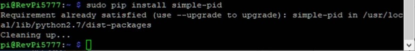
Nearly all Python scripts have an “import” section at the beginning. This section tells the interpreter which libraries to use for the script. Python extensively uses libraries. I’m convinced that this concept of having a minimal set of common language elements and leaving the rest to libraries contributed to by a huge worldwide community is the core of the success of this language. It’s all about “Swarm intelligence”. If you have a particular problem, google for a Python lib, and there is a great chance to find it. That’s the case with the PID control algorithm. I found, e.g. “simple-pid”.  Before you can use a library, most of the time you need to install it on your system. I use my SSH session (PuTTY) to enter the shell command “sudo pip install simple-pid” (in the following screen dump the lib has already been installed):

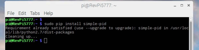
By the way: I could also have used a terminal window on the RevPi desktop to do so:

“pip” is a great tool which tries to get the library from a central repository of the Python organisation and then install it on your system. Above we already have installed “python3-revpimodio2” and “revpipyload” from the KUNBUS repository using the Linux apt-get command.

If the installation has been successful, your expression to import these libs will not result in an error message:

>>> from simple_pid import PID

>>> import revpimodio2

Okay, now let’s write the script. We use the Python shell’s menu ”File” -> “New File” to open a new empty editor window and enter the import expressions as the first two lines. You will find that the editor tries to help you by marking Python keywords immediately in a different colour.

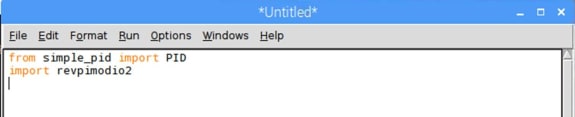
I hate losing time by a system crash, so I better save this file from time to time. You find the command under “File” -> “Save”. For following this instruction I recommend saving it to the “/home/pi” directory with name “myplc.py”.

Many libraries will be found on GitHub, and there you will also find documentation. Look here for our library. There we also find an example which makes it easy to understand the usage instantaneously. We follow the example and create an instance “TempController” of the PID object class by the expression:

TempController = PID(1,0.1,0.0, setpoint=250, output_limits=(0,100))

The documentation for the class init call names the function parameters:

• Kp=1.0 value for the proportional gain (better called “controller gain”)
• Ki=0.1 value for the integral gain
• Kd=0.0 value for the derivative gain
• setpoint=250 initial setpoint that the PID will try to achieve (in our case 25 °C temperature *10)
• sample_time=0.1 the time in seconds which the controller should wait before generating a new output value. The PID works best when it is constantly called (e.g. during a loop), but with a sample time set so that the time difference between each update is (close to) constant. If set to None, the PID will compute a new output value every time it is called. I use 100 ms because with the 10W heater I will get very slow temperature changes.
• output_limits=(0, 100) The initial output limits to use, given as an iterable with two elements, for example: (lower, upper). The output will never go below the lower limit or above the upper limit. 

  rpi.io.PWM_heater1.value = int(pwm)
  rpi.io.PWM_heater2.value = int(pwm)
  ​

  Either of the limits can also be set to None to have no limit in that direction. Setting output limits also avoids integral windup, since the integral term will never be allowed to grow outside of the limits. In our case, we want to use the PWM values from 0% to 100%.
• auto_mode=True This is the default (PID controller enabled)
• proportional_on_measurement=False Whether the proportional term should be calculated on the input directly rather than on the error (which is the traditional way). Using proportional-on-measurement avoids overshoot for some types of systems. I use the default = False.

If you are not familiar with PID control algorithms, you may consult this page for further explanation of the tuning parameters Kp, Ki and Kd. We will not be able to predict these tuning values and need to set them by testing the control behaviour (see later in this article).

We also need to get an instance of the revpimodio class. So we use the documentation on the revpimodio web pages to find the init-call for it:

rpi = revpimodio2.RevPiModIO(autorefresh=True)

There are three functions we need to call cyclically to operate the PID controller:

The first one is getting the current temperature from the process image:

Temp = rpi.io.Temp10.value

The second one is the calculation of the PID output value:

pwm = TempController(Temp)

The last one is setting the PWM outputs to the calculated value by writing to the process image:

As the PWM value in the process image is an unsigned integer, we need to convert the PID output with the function “int()”. I have put these four lines in an endless loop using Python’s while loop with the argument “True”. If you are not familiar with Python, please note that in Python there are no {} pairs to group code. Code is grouped by using the “white space” (=indentation) which you can see before the four statements inside the while loop.

As we have a multi-tasking Linux system, we do not want to block the CPU by having a tight endless loop in our task. So I use the library “time” and the function “sleep(n)” to give the loop a 0.05-second pause. To have debug-outputs every second, I also added a counter variable which is incremented every cycle of the loop up to 20 and then reset to 0 after printing the input and output values.

Here is the complete program:

from simple_pid import PID
import revpimodio2
import time

TempController = PID(5,0.13,10.5, sample_time=0.1, setpoint=400, output_limits=(0,100))
rpi = revpimodio2.RevPiModIO(autorefresh=True)
n=0
while True:
    Temp = rpi.io.Temp10.value
    pwm = TempController(Temp)
    rpi.io.PWM_heater1.value = int(pwm)
    rpi.io.PWM_heater2.value = int(pwm)
    n +=1
    if n==20:
        n=0
        print(Temp, int(pwm))
    time.sleep(0.05)

If you start this script with <F5> or via menu “Run” -> “Run Module” you can see the cyclical value print on the Python shell window. You can stop the execution by pressing CTRL-C.

Now it’s time to experiment with the tuning values. They will certainly depend on the physical feedback between the heat source and temperature sensor. I want to make this feedback close. So I chose a small distance between the sensor and the light bulbs:

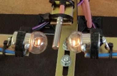
I could also put them in a case or aluminium foil which catches the heat.

However, in my case, with 2 x 10 W heater and setpoint temperatures around 40°C, I could manage to adjust the three tuning parameters to reach a nearly perfect control. To get there, I started by setting Ki and Kd to 0. Taking values for Kp of 1, 5, 10 and 20, I observed a stable end temperature for 10. This means: For each 0.1°C deviation under the setpoint, the control function returns 10% more PWM on time. Using a value of 20 did result in more than 1°C oscillations. I then took half of the stable value 10, i.e. 5 for Kp. This results in a very stable end temperature, which has a negative offset of the setpoint – instead of reaching 40°C, the temperature only went up to about 39°C. I started to very slowly raise Ki, which kind of compensating the offset but raises oscillation. With a value of 0.13, I have got a stable 1°C peak to peak oscillation around the setpoint of 40°C. Raising Kd the controller kind of “injects” short pulses to a higher or lower PWM value. This does reduce oscillation. I finally got a value around 10 for Kd with an oscillation of +/- 0.1 °C (which is the overall precision of the temperature measurement). Here you can see the result of tuning:

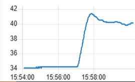
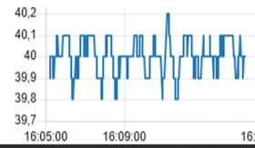
At 15:57 the controller was switched on at an ambient temperature of 34 °C (yes, I do have a climate change in my office!). At 15:59 (after 2 minutes), the temperature reached a stable temperature of 40 °C (setpoint). The second picture shows the very small oscillation around the setpoint.

If your text output shows an acceptable control loop, you can go on to the next step: Using MQTT and Node-Red to build a little GUI for our heater controller to get nice charts like the above time courses. But that’s the content of part 4.