CNC Router Process Optimisation with ST IO-Link Solutions Part 3: Software, Processing Data & Final Testing

Writing a Python script to parse log files, performing a number of machining jobs to gather data and exploring the results.

In part two of this series we designed a suitable enclosure to house the ST STEVAL-BFA001V2B sensor board, that would protect the sensitive electronics from coolant mists and metal chips. The assembly was installed onto the CNC machine and some preliminary data was gathered to test basic operation of the measurement solution.

In this post, we’ll be writing a Python script to wrangle the human-readable log files produced by ST’s STEVAL-IDP005Vx-GUI 2.0 Windows application, running a number of machining jobs with different parameters to gather data and seeing how the data reflects the machining results.

Gathering Data

To start, we needed to gather data from a machining job so that we had something to work with. We opted to machine a simple cuboid out of aluminium, that would require a ramp into the material to mill the outer edges, with short plunges at the final depth to create holding tabs. The top surface would then have a finishing pass to take the part down to size.

Each run had the spindle RPM kept constant and coolant enabled, with only the feed rate changing per run — this was first set at 700mm/minute and we performed a run at 50% feed (350mm/min) and 125% (875mm/minute).

To simulate a worst-case scenario we ran the same machining job with the same feed rate and an increased step-down distance in a deliberate attempt to cause severe chatter in the part.

Handling the Log Files

Instead of writing an entire custom application that interfaced with the ST IO-Link master, we opted to rely on the “STEVAL-IDP005Vx-GUI 2.0” Windows application.

Measures Added 1/12/2022 3:48:56 PM

RMS Speed: X: 0.03 | Y: 0.04 | Z: 0.06 [mm/s]
ACC PEAK:  X: 0.43 | Y: 0.38 | Z: 0.47 [m/s2]
Pressure: 1031.20 mBAR
Humidity: 45.39 %RH
Environmental temperature: 25.36 °C
Sound pressure level: 42.00 dB



Measures Added 1/12/2022 3:49:01 PM

| [Hz] 	| X 	| Y 	| Z 	|
| 0 	| 0 	| 0 	| 0 	| 
| 13.08789 	| 0.002221676 	| 0.003107379 	| 0.003380591 	| 
| 26.17578 	| 0.003749868 	| 0.004776487 	| 0.006495491 	| 
| 39.26367 	| 0.008637507 	| 0.01139208 	| 0.01555778 	| 

The application provides logging features that emit human-readable text files which are not suited for automated processing; additional work to convert the data into a more machine-readable format first needed to be done. Each log file also contains both FFT sample data and regular sensor data, which further complicates things.

To handle these files we wrote a Python script that scans through the file to split out each chunk (regular readings and FFT data) into separate CSV files.

The first step is to load in the file, which is done using a with open statement — this provides a context manager that safely handles opening the file for us to use. All the lines are then read into a list, and then iterated over in a for loop. The advantage of using a context manager is that the file handle is released no matter what happens, even if the program unexpectedly exits.

if "Measures Added" in line or "Created:" in line:
				date_time_string = re.search(datetime_pattern, line)
				if date_time_string:
					block_timestamp = time.mktime(datetime.datetime.strptime(date_time_string.group(0), "%m/%d/%Y %H:%M:%S %p").timetuple())
					print("Block timestamp {}".format(block_timestamp))

As each reading is prefixed with the same string — such as “Measures Added” for the timestamp, “RMS Speed” for the speed measurements, “ACC PEAK” for the peak acceleration values and so on — we can easily match based on these strings to split out the data.

block_timestamp = time.mktime(datetime.datetime.strptime(date_time_string.group(0), "%m/%d/%Y %H:%M:%S %p").timetuple())

The first step is to parse the date and time from a line. This is done using a regular expression pattern of ([0-9]+(/[0-9]+)+).*([0-9]+(:[0-9]+)+).*[a-zA-Z]+ that returns a string from any line containing “Measures Added” or “Created:”. To convert the string into a Python datetime object, the strptime() function is employed with a format code that matches the layout in the log file. This is then parsed into a numeric timestamp using time.mktime() ready for including with other data.

To parse numeric data out from a line, another regex pattern is employed to extract readings as floating-point values. As some entries such as the RMS speed include multiple data points per line, the Python function re.finditer() is employed to iterate over the line with the regex pattern. This returns an object that contains all the matches which are again iterated over, inserted into a dictionary and then written to the CSV file.

if "| [Hz] 	|" in line:
	fft_data_block = True

if fft_data_block and "| [Hz] 	|" not in line and line != "\n":
	fft_values = re.finditer(floating_point_pattern, line)
	fft_list = []
	if fft_values:
		for value in fft_values:
			fft_list.append(value.group(0))

			fft_data_line['frequency'] = fft_list[0]
			fft_data_line['x'] = fft_list[1]
			fft_data_line['y'] = fft_list[2]
			fft_data_line['z'] = fft_list[3]
			fft_data_line['timestamp'] = block_timestamp

			print("Writing FFT CSV record")
			fft_writer.writerow(fft_data_line)

Logic is implemented to handle the FFT data block so that the output is sent to a separate CSV file. The application first checks for “| [Hz] |” in the current line, sets the fft_data_block variable to true, and then iterates over the next line. If the fft_data_block variable is true, the line does not contain “| [Hz] |” and is not a newline then processing begins.

Just as before, each data point is extracted using a regex pattern match. The values are put into a dictionary, then written out to the CSV file.

Data Processing

We ran our Python script over each of the resulting log files from the four machining runs, which produced a number of CSV files. Each was then opened in Excel and graphs of the data points plotted.

To compare the machining jobs we captured data for each run, took images of the same face of each finished part under a microscope, and also made some observations on how the job “felt” — such as observed noise levels, moments of particularly bad chatter and overall part finish.

Throughout our tests we found that the sound pressure levels across all the runs would hit a maximum of 60 dB and no higher — the microphone has an AOP (Acoustic Overload Point) of 122.5 dBSPL and a 64 dB signal-to-noise ratio, and thus should be able to process the noise of the CNC router. This issue could be alleviated by providing some form of acoustic dampening around the microphone beyond what we have provided.

Another issue we found with the gathered data was the low sample rate at which the sensor was polled for readings, due to the inability to configure this in the provided demonstration application — writing custom firmware for the IO-Link master and sensor, and some custom PC software would allow for improvements upon the sample rate. However, the data gathered demonstrates that it would be worth further investigation to improve the sample rate.

We opted to focus on the acceleration measurements produced, as our theory was that these would represent chatter/machine movements reasonably well. We predicted that lots of chatter would produce a fairly spiky acceleration graph as the tool skips through the material, as opposed to smoothly cutting through.

Each image of the resulting surface finish was taken looking at the same face of each part, which had the worst finish across all five machined surfaces.

Run 1 - 50% Feedrate

Our first machining job was performed at a 50% feed rate (350mm/minute). As can be seen in the microscope image above, chatter is evident in the finished part and the machine subjectively made lots of noise when performing the cut.

The resulting graph of acceleration shows prominent spikes throughout the middle of the cutting process, suggesting that chatter of the tool was occurring. The first part of the graph shows a smooth acceleration across all three axes where the machine begins the cut. Similarly, the end of the graph shows another smooth acceleration as the machine performs the final facing cut and the job finishes.

The average amplitude of the graph is also quite high, with peaks regularly hitting and occasionally exceeding 40 units.

Run 2 - 100% Feedrate

The next machining job was performed at 100% feed rate (700mm/min), with all other process parameters unchanged. As before chatter is evident but to a lesser degree when compared to the 50% feedrate run. The machine also subjectively produced less chatter related noise throughout the milling process.

When the cut is underway (towards the right-hand side of the chart) peaks are again seen but to a lesser extent when compared with before — suggesting that less chatter was taking place during the cuts. The peak amplitude is on average lower, with a value of 40 being achieved only three times.

Run 3 - 125% Feedrate

Our third machining job was performed at a feed rate of 125%, or 825mm/minute. Again, no other process parameters were changed. Chatter is fairly minimal on this part and the noise from the machine was reduced.

Interestingly, the graph of acceleration on each axis showed a spiky appearance, much like the 50% feedrate run. Peaks of 40 units and above are common, which based upon our theory suggests lots of chatter took place — however the finish on the part surfaces does not support this.

This discrepancy could have been caused by a lack of data being available due to the sampling rate of the sensor or due to other reasons. For example, an FFT of this machining run, as shown above, shows lots of high-frequency content and it is possible there was some sort of interaction between parts of the machine that did not result in chatter, but resulted in a noisy data output.

Run 4 - 100% Feedrate, increased step down

To create a worst-case scenario we kept the same spindle speed of 13000 rpm and feedrate of 700mm/minute, but increased the step down from 1 mm to 2.5 mm. This created a greatly increased load on the tool, increasing the chance that chatter would occur.

This run did indeed fulfil our desired outcome of creating lots of chatter, however, it required hitting the CNC router emergency stop button due to chip welding — limiting the amount of data that could be gathered. Again, with a custom solution involving different firmware and software, the sensor sample rate could be increased to gather data at shorter intervals.

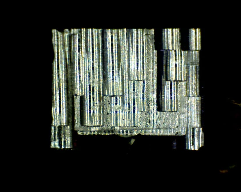
As can be seen in the above image, severe chatter is present. The machine produced lots of noise, vibration and eventually succumbed to chip welding on the end mill. Evidence of overheating is present in the workpiece, with molten aluminium being spread throughout the cut path.

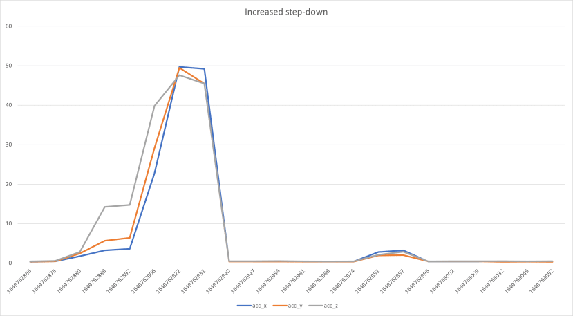
The graph of this run contained a limited amount of acceleration data. As can be seen from the data, a lot of high amplitude machine vibration was present that was almost constant across the short duration of the machining job. The highest amplitude achieved peaked at 50 units, and the average value was close to this peak.

Additionally, the FFT data shows that lots of broadband high amplitude vibration across all axes were present, indicating that the machining operation was not smooth.

Demonstration Video

Final Remarks

This project has explored a range of issues surrounding CNC routing and machining processes, and then looked at the use of IO-Link development kits from ST Microelectronics to demonstrate a machinery monitoring solution that can augment the eyes and ears of an experienced machinist.

With some further work, this could be turned into a viable solution to provide insights into machining processes such as CNC routing or milling, where chatter and other issues can quite quickly destroy a part and tool. Such a solution could be used to enable process optimisation, together with alerting and automatically halting the process when a failure condition has been detected.