Building an Amplifier Test Set with Analog Discovery 2 and Raspberry Pi 4 Part 2: Software
Follow article
 Dave from DesignSpark
How do you feel about this article? Help us to provide better content for you.
Dave from DesignSpark
Thank you! Your feedback has been received.
Dave from DesignSpark
There was a problem submitting your feedback, please try again later.
Dave from DesignSpark
What do you think of this article?
Using the multifunction instrument together with a Raspberry Pi 4 to create a standalone programmable audio amplifier test set.
In Part 1 in this series, we outlined the basic operation of the amplifier test set, before going on to take a first look at the Analog Discovery 2 and provided software, along with the other hardware components that we planned to use. In this post, we take a look at the software in a little more detail, via simple examples that demonstrate how we might develop custom test functionality.
Typical test scenarios
When testing audio amplifiers typical measurements include:
- Gain
- Frequency response
- Total harmonic distortion (THD)
- Crosstalk in amplifiers with >1 channel
- Phase
- DC level
In addition to such generalised measurements which are common across amplifier equipment, there will also be tests that are performed as part of the servicing procedure for a particular amplifier, which call for a specific input signal to be provided and a desired output signal to be observed. The latter might be used in ascertaining whether a component or part of the circuit is not functioning correctly, or perhaps used as part of alignment procedures, e.g. biasing.
With the above in mind it is clear to see the benefit of specialised audio test equipment, which may not only be able to quickly calculate things such as THD, but also automate tasks such as setting up an appropriate signal generation for the amplifier input.
Hardware setup
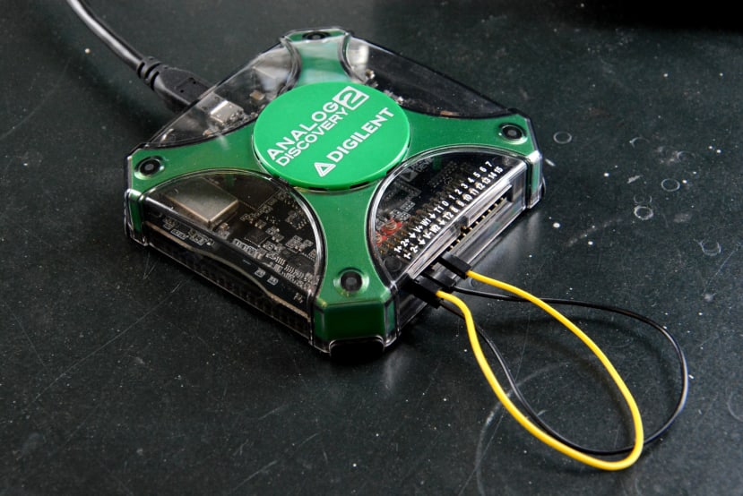
For the purposes of this post and for convenience when it later comes to developing some simple example test cases, we will have the Analog Discovery 2 connected to a laptop running Ubuntu 20.04. In a future post, we’ll switch to using a Raspberry Pi 4 that is integrated into an enclosure with the other components.
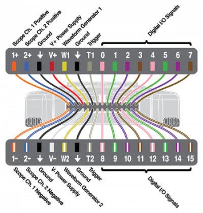
Above we can see the pinout for the Analog Discover 2 I/O. For the simple examples covered here, we will simply connect the output of waveform generator 1 to scope channel 1 positive input. Since the scope channels are differential, the channel 1 negative input is then also tied to ground.
WaveForms
As mentioned in Part 1, software support for the Analog Discovery 2 is provided courtesy of the WaveForms virtual instrument suite. We followed the Getting Started Guide for Linux, but note that Mac and Windows are also supported.
First, we needed to download the Adept 2 runtime, followed by WaveForms itself. These were then installed with:
$ sudo dpkg -i digilent.adept.runtime_2.21.3-amd64.deb

$ sudo dpkg -i digilent.waveforms_3.16.3_amd64.deb
The second install resulted in an error since libqt5scripttools5 was not installed on our system, but such dependency errors are easily remedied with:
$ sudo apt -f installAt this point we could now start WaveForms with:
$ waveforms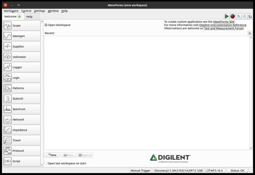
When the application loads we are presented with the Welcome tab, which allows us to open a recent workspace and via a column of buttons down the left-hand side, to load up one or more virtual instruments. The Getting Started Guide walks us through taking our first measurement, using the Wavegen and Scope instruments.
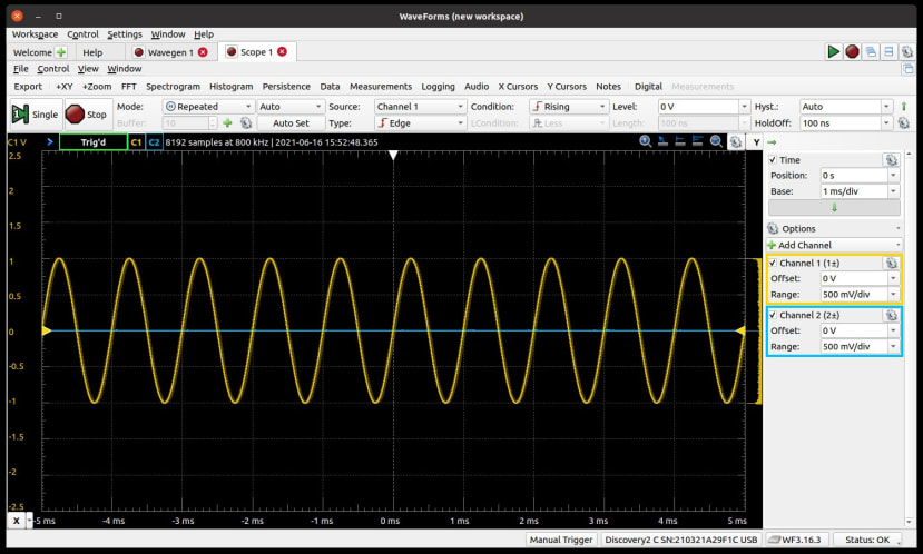
With this, we generate a 1kHz sine wave and then loop this back and display the signal on the scope.
Next, we’ll take a look at something a little more advanced and that might prove particularly useful for our application of testing audio amplifiers and measuring their performance.
The Digilent website includes an example that shows how to measure harmonics in a signal.
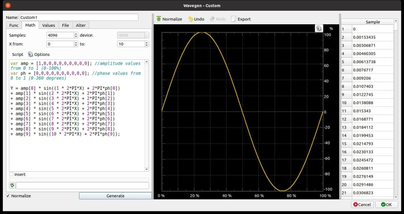
We start again by adding a Wavegen virtual instrument, but this time the Custom mode is selected, we navigate to the Math tab and then we add the code shown below.
var amp = [1,0,0,0,0,0,0,0,0,0]; //amplitude values from 0 to 1 (0-100%)
var ph = [0,0,0,0,0,0,0,0,0,0]; //phase values from 0 to 1 (0-360 degrees)
Y = amp[0] * sin((1 * 2*PI*X) + 2*PI*ph[0])
+ amp[1] * sin((2 * 2*PI*X) + 2*PI*ph[1])
+ amp[2] * sin((3 * 2*PI*X) + 2*PI*ph[2])
+ amp[3] * sin((4 * 2*PI*X) + 2*PI*ph[3])
+ amp[4] * sin((5 * 2*PI*X) + 2*PI*ph[4])
+ amp[5] * sin((6 * 2*PI*X) + 2*PI*ph[5])
+ amp[6] * sin((7 * 2*PI*X) + 2*PI*ph[6])
+ amp[7] * sin((8 * 2*PI*X) + 2*PI*ph[7])
+ amp[8] * sin((9 * 2*PI*X) + 2*PI*ph[8])
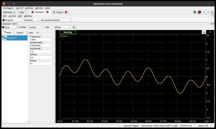
+ amp[9] * sin((10 * 2*PI*X) + 2*PI*ph[9]);If we next select Generate, this will again output a sine wave, but we can distort this by changing the amplitude and phase values. E.g. setting the former too:
var amp = [1,1,0,0,0,0,1,0,0,0];Gives us the following Wavegen output and scope plot.
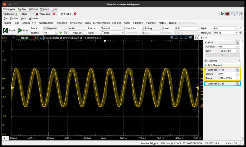
The provided harmonics example has us set the following test vector in the generator:
var amp = [1,0,0.33,0,0.2,0,0.14,0,0.11,0];Next setting up the scope and its FFT function appropriately, which gives us the following time and frequency domain plots.
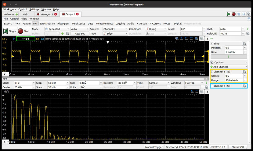
This clearly shows the base frequency and harmonics, allowing us to measure the amplitude of the latter with respect to the former.
At this point, we can save the custom Wavegen settings inside this virtual instrument, and from the Welcome tab, we can select to save the workspace. In this way, we can easily create and recall configurations for performing different tests, which may be generic, or perhaps specific to a particular amplifier and its servicing procedures. We could also go one step further and use the integrated script editor to automate functions and examples can be found in this blog post.
However, next let’s take a look at the SDK and how this can be used to create fully custom applications, that have just the functionality that you require and nothing more.
WaveForms SDK
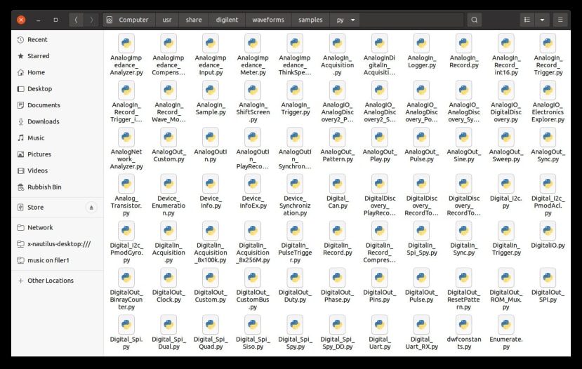
The WaveForms application uses a runtime to communicate with the Analog Discovery 2 and this also provides a public API for custom applications. Code samples that make use of this are provided for Python, C, C# and Visual Basic. We’ll be using Python and in the above screenshot, we can see that there are plenty of examples to help get us up and running — a total of 76 in fact!
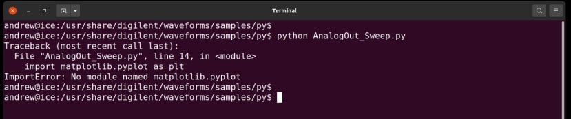
If we try to run these we may encounter errors if a Python dependency is missing. For example, upon executing AnalogOut_Sweep.py it was discovered that we need the Matplotlib module. It turned out that on Ubuntu 20.04 there wasn’t a package for this for the default Python 2.7, but there was for Python 3 and this was already installed. Fortunately, the samples appear to have been written with both Python versions in mind and so the simplest fix was to run with python3 instead.
Of course, another possibility might have been to install Matplotlib for Python 2.7 via PyPy (pip), but we really should be using Python 3 in any case.
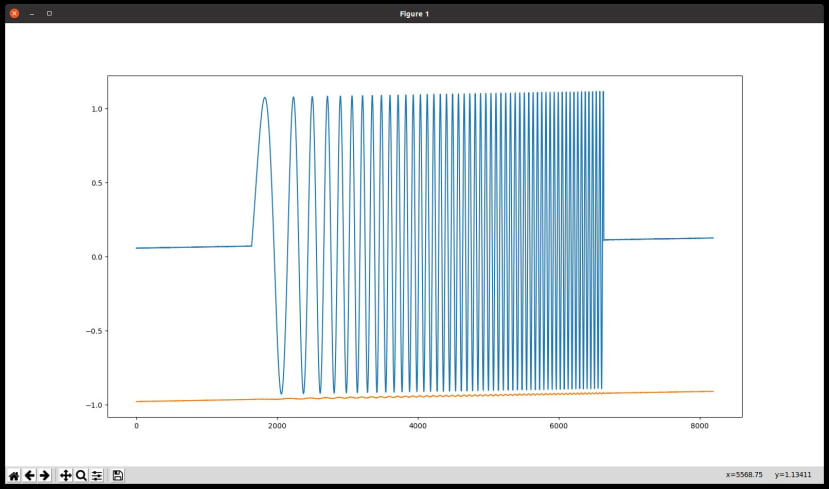
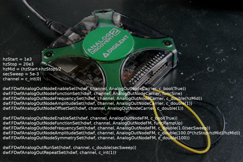
Back to running our example with Python 3 and above we can see the plot that was generated.
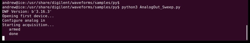
The terminal output can be seen above. Let’s next take a look at the code itself.
hzStart = 1e3

hzStop = 20e3

hzMid = (hzStart+hzStop)/2

secSweep = 5e-3

channel = c_int(0)


dwf.FDwfAnalogOutNodeEnableSet(hdwf, channel, AnalogOutNodeCarrier, c_bool(True))

dwf.FDwfAnalogOutNodeFunctionSet(hdwf, channel, AnalogOutNodeCarrier, funcSine)

dwf.FDwfAnalogOutNodeFrequencySet(hdwf, channel, AnalogOutNodeCarrier, c_double(hzMid))

dwf.FDwfAnalogOutNodeAmplitudeSet(hdwf, channel, AnalogOutNodeCarrier, c_double(1))

dwf.FDwfAnalogOutNodeOffsetSet(hdwf, channel, AnalogOutNodeCarrier, c_double(1))


dwf.FDwfAnalogOutNodeEnableSet(hdwf, channel, AnalogOutNodeFM, c_bool(True))

dwf.FDwfAnalogOutNodeFunctionSet(hdwf, channel, AnalogOutNodeFM, funcRampUp)

dwf.FDwfAnalogOutNodeFrequencySet(hdwf, channel, AnalogOutNodeFM, c_double(1.0/secSweep))

dwf.FDwfAnalogOutNodeAmplitudeSet(hdwf, channel, AnalogOutNodeFM, c_double(100.0*(hzStop-hzMid)/hzMid))

dwf.FDwfAnalogOutNodeSymmetrySet(hdwf, channel, AnalogOutNodeFM, c_double(100))


dwf.FDwfAnalogOutRunSet(hdwf, channel, c_double(secSweep))

dwf.FDwfAnalogOutRepeatSet(hdwf, channel, c_int(1))
We’ll fast-forward past the module imports and opening the device. Above we can see some variables being declared, and then an analogue output — arbitrary waveform generator — is set up using these. The functions and their parameters are fairly self-explanatory.
hzRate = 1e6

cSamples = 8*1024

rgdSamples1 = (c_double*cSamples)()

rgdSamples2 = (c_double*cSamples)()

sts = c_int()


print("Configure analog in")

dwf.FDwfAnalogInFrequencySet(hdwf, c_double(hzRate))

dwf.FDwfAnalogInChannelRangeSet(hdwf, c_int(-1), c_double(4))

dwf.FDwfAnalogInBufferSizeSet(hdwf, c_int(cSamples))

dwf.FDwfAnalogInTriggerSourceSet(hdwf, trigsrcAnalogOut1)

dwf.FDwfAnalogInTriggerPositionSet(hdwf, c_double(0.3*cSamples/hzRate)) # trigger position at 20%, 0.5-0.3


print("Starting acquisition...")

dwf.FDwfAnalogInConfigure(hdwf, c_int(1), c_int(1))
Then it’s much the same again, albeit this time setting up an analogue input. Following which acquisition is started and upon completion, samples are copied to buffers, the device is closed and the results are plotted.
So this much like our earlier examples using the Wavegen and Scope virtual instruments in the WaveForms application.
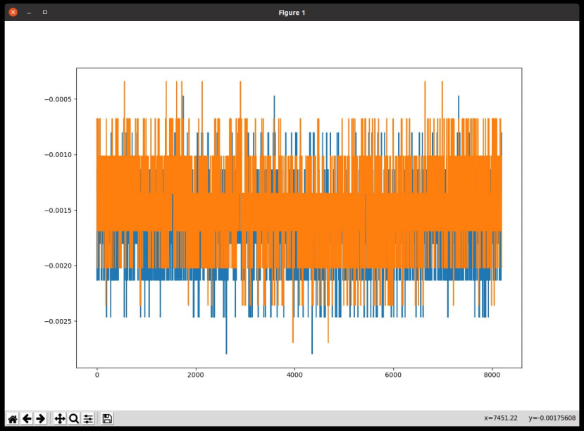
Just to prove that we are not cheating, above can be seen the plot generated when the yellow wire that connects waveform 1 output to scope channel 1 input is disconnected — all we get is noise.
There is also an SDK Reference Manual that makes it that little bit easier to understand the samples and all the API functions. This covers API basics, such as the correct sequence of steps to discover connected devices — you may have more than one plugged in — open a connection and configure instruments etc.
The API functions are documented in detail and organised into the following groups:
- Device Enumeration
- Device Control
- AnalogIn (oscilloscope)
- AnalogOut (AWG)
- AnalogIO (acquire/drive various analogue signals)
- DigitalIn (logic analyzer)
- DigitalOut (pattern generator)
- DigitalIO (acquire and drive digital I/O signals)
- System (obtain basic system information)
Summing up
From this simple vendor-provided SDK sample we can see how custom applications might easily be created that combine signal generation for an audio amplifier input, while also plotting the signal output by the device under test, therefore allowing us to characterise it. Our application may additionally sequence a whole set of equipment-specific tests, give us a simple pass/fail indication, log the results to a file and perhaps even take an equipment serial number to record against these. There is a lot of functionality that could be developed so as to speed up testing, while also reducing the possibility of errors resulting from incorrect test equipment setup.
In the next post, we’ll assemble the amplifier test set hardware platform, which will utilise a Raspberry Pi 4 for the host computer, with a Raspberry Pi Touch Screen display, plus of course the dummy load, and some simple physical controls for ease-of-use.